Detect objects using MobileNet SSD

In this tutorial, you'll use machine learning to build a system that can recognize and track multiple objects in your house through a camera - a task known as object detection. Adding sight to your embedded devices can make them see the difference between poachers and elephants, count objects, find your lego bricks, and detect dangerous situations. In this tutorial, you'll learn how to collect images for a well-balanced dataset, how to apply transfer learning to train a neural network and deploy the system to an edge device.

At the end of this tutorial, you'll have a firm understanding of how to do object detection using Edge Impulse.

There is also a video version of this tutorial:

You can view the finished project, including all data, signal processing and machine learning blocks here: Tutorial: object detection.

Running on a microcontroller?

We recently released a brand-new approach to perform object detection tasks on microcontrollers, FOMO, if you are using a constraint device that does not have as much compute, RAM, and flash as Linux platforms, please head to this end-to-end tutorial: Detect objects using FOMO

Alternatively, if you only need to recognize a single object, you can follow our tutorial on Adding sight to your sensors - which performs image classification, hence, limits you to a single object but can also fit on microcontrollers.

You can view the finished project, including all data, signal processing and machine learning blocks here: Tutorial: object detection.

1. Prerequisites

For this tutorial, you'll need a supported device.

If you don't have any of these devices, you can also upload an existing dataset through the Uploader - including annotations. After this tutorial you can then deploy your trained machine learning model as a C++ library and run it on your device.

2. Building a dataset

In this tutorial we'll build a model that can distinguish between two objects on your desk - we've used a lamp and a coffee cup, but feel free to pick two other objects. To make your machine learning model see it's important that you capture a lot of example images of these objects. When training the model these example images are used to let the model distinguish between them.

Capturing data

Capture the following amount of data - make sure you capture a wide variety of angles and zoom level. It's fine if both images are in the same frame. We'll be cropping the images later to be square so make sure the objects are in the frame.

  • 30 images of a lamp.

  • 30 images of a coffee cup.

You can collect data from the following devices:

Or you can capture your images using another camera, and then upload them by going to Data acquisition and clicking the 'Upload' icon.

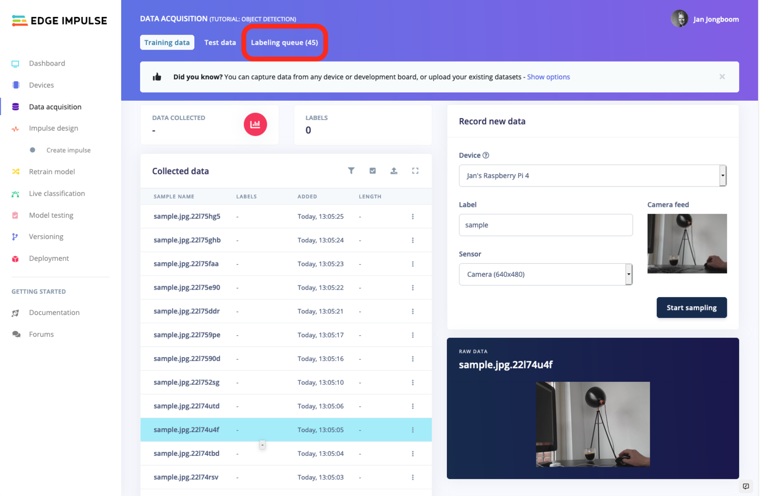
With the data collected we need to label this data. Go to Data acquisition, verify that you see your data, then click on the 'Labeling queue' to start labeling.

Collected data, now let's label the data with the labeling queue.

No labeling queue? Go to Dashboard, and under 'Project info > Labeling method' select 'Bounding boxes (object detection)'.

Labeling data

The labeling queue shows you all the unlabeled data in your dataset. Labeling your objects is as easy as dragging a box around the object, and entering a label. To make your life a bit easier we try to automate this process by running an object tracking algorithm in the background. If you have the same object in multiple photos we thus can move the boxes for you and you just need to confirm the new box. After dragging the boxes, click Save labels and repeat this until your whole dataset is labeled.

AI-Assisted Labeling

Use AI-Assisted Labeling for your object detection project! For more information, check out our blog post.
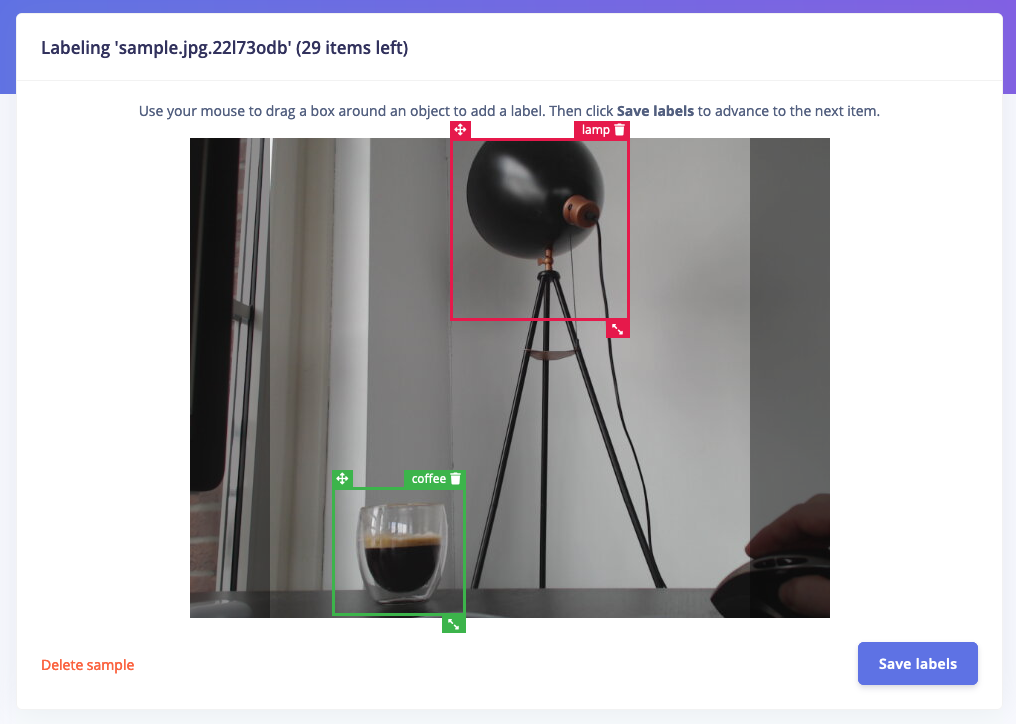
Labeling multiple objects with the labeling queue. Note the dark borders on both sides of the image, these will be cut off during training, so you don't have to label objects that are located there.

Afterwards you should have a well-balanced dataset listed under Data acquisition in your Edge Impulse project.

Rebalancing your dataset

To validate whether a model works well you want to keep some data (typically 20%) aside, and don't use it to build your model, but only to validate the model. This is called the 'test set'. You can switch between your training and test sets with the two buttons above the 'Data collected' widget. If you've collected data on your development board there might be no data in the testing set yet. You can fix this by going to Dashboard > Perform train/test split.

3. Designing an impulse

With the training set in place you can design an impulse. An impulse takes the raw data, adjusts the image size, uses a preprocessing block to manipulate the image, and then uses a learning block to classify new data. Preprocessing blocks always return the same values for the same input (e.g. convert a color image into a grayscale one), while learning blocks learn from past experiences.

For this tutorial we'll use the 'Images' preprocessing block. This block takes in the color image, optionally makes the image grayscale, and then turns the data into a features array. If you want to do more interesting preprocessing steps - like finding faces in a photo before feeding the image into the network -, see the Building custom processing blocks tutorial. Then we'll use a 'Transfer Learning' learning block, which takes all the images in and learns to distinguish between the two ('coffee', 'lamp') classes.

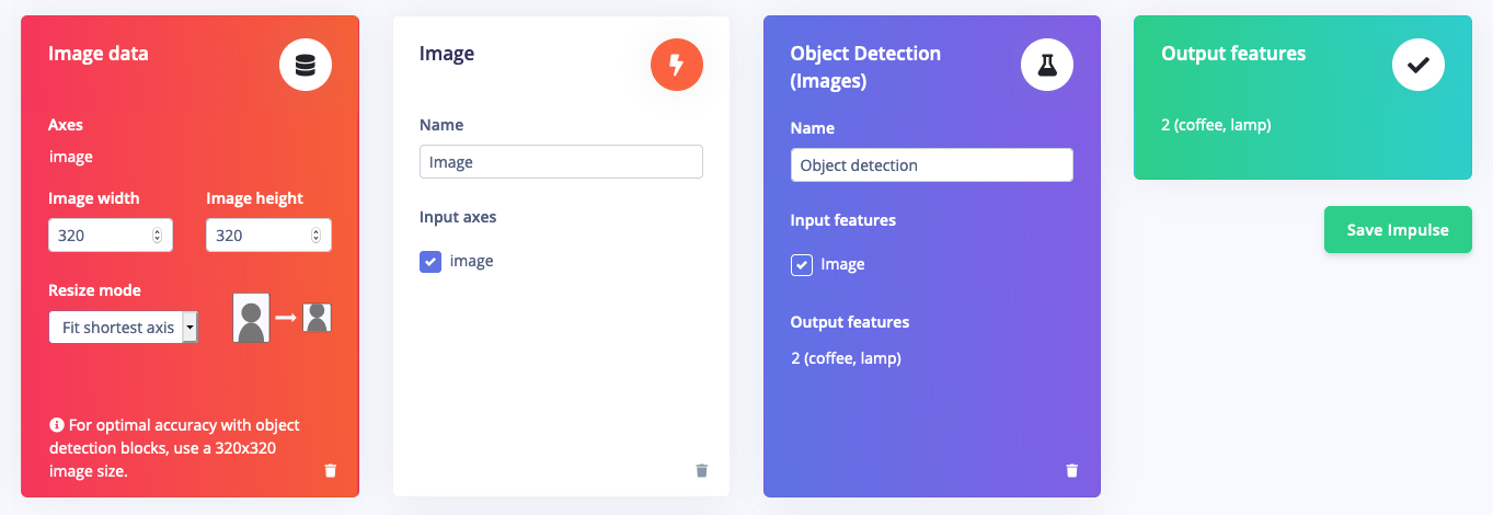
In the studio go to Create impulse, set the image width and image height to 320, the 'resize mode' to Fit shortest axis and add the 'Images' and 'Object Detection (Images)' blocks. Then click Save impulse.

Designing an impulse

Configuring the processing block

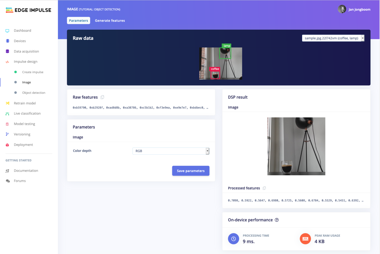
To configure your processing block, click Images in the menu on the left. This will show you the raw data on top of the screen (you can select other files via the drop down menu), and the results of the processing step on the right. You can use the options to switch between 'RGB' and 'Grayscale' mode, but for now leave the color depth on 'RGB' and click Save parameters.

Configuring the processing block.

This will send you to the 'Feature generation' screen. In here you'll:

  • Resize all the data.

  • Apply the processing block on all this data.

  • Create a 3D visualization of your complete dataset.
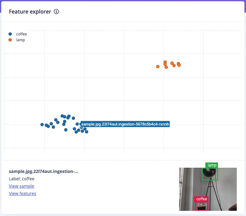
Click Generate features to start the process.

Afterwards the 'Feature explorer' will load. This is a plot of all the data in your dataset. Because images have a lot of dimensions (here: 320x320x3=307,200 features) we run a process called 'dimensionality reduction' on the dataset before visualizing this. Here the 307,200 features are compressed down to just 3, and then clustered based on similarity. Even though we have little data you can already see the clusters forming (lamp images are all on the left, coffee all on the right), and can click on the dots to see which image belongs to which dot.

The feature explorer visualizing the data in the dataset. Clusters that separate well in the feature explorer will be easier to learn for the machine learning model.

Configuring the transfer learning model

With all data processed it's time to start training a neural network. Neural networks are a set of algorithms, modeled loosely after the human brain, that are designed to recognize patterns. The network that we're training here will take the image data as an input, and try to map this to one of the three classes.

It's very hard to build a good working computer vision model from scratch, as you need a wide variety of input data to make the model generalize well, and training such models can take days on a GPU. To make this easier and faster we are using transfer learning. This lets you piggyback on a well-trained model, only retraining the upper layers of a neural network, leading to much more reliable models that train in a fraction of the time and work with substantially smaller datasets.

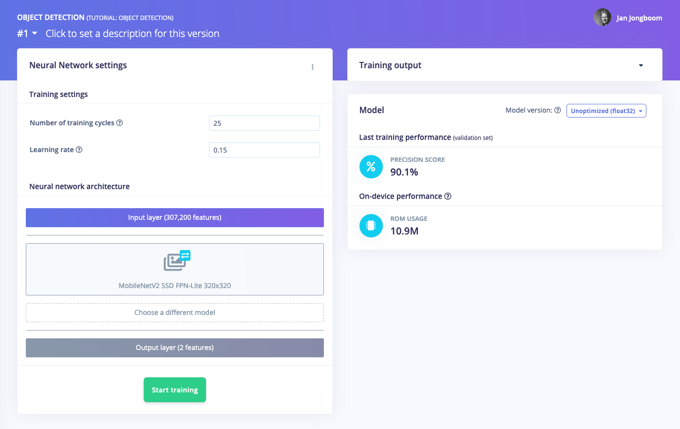
To configure the transfer learning model, click Object detection in the menu on the left. Here you can select the base model (the one selected by default will work, but you can change this based on your size requirements), and set the rate at which the network learns.

Leave all settings as-is, and click Start training. After the model is done you'll see accuracy numbers below the training output. You have now trained your model!

A trained model showing the precision score. This is the COCO mean average precision score, which evaluates how well the predicted labels match your earlier labels.

4. Validating your model

With the model trained let's try it out on some test data. When collecting the data we split the data up between a training and a testing dataset. The model was trained only on the training data, and thus we can use the data in the testing dataset to validate how well the model will work in the real world. This will help us ensure the model has not learned to overfit the training data, which is a common occurrence.

To validate your model, go to Model testing and select Classify all. Here we hit 92.31% precision, which is great for a model with so little data.
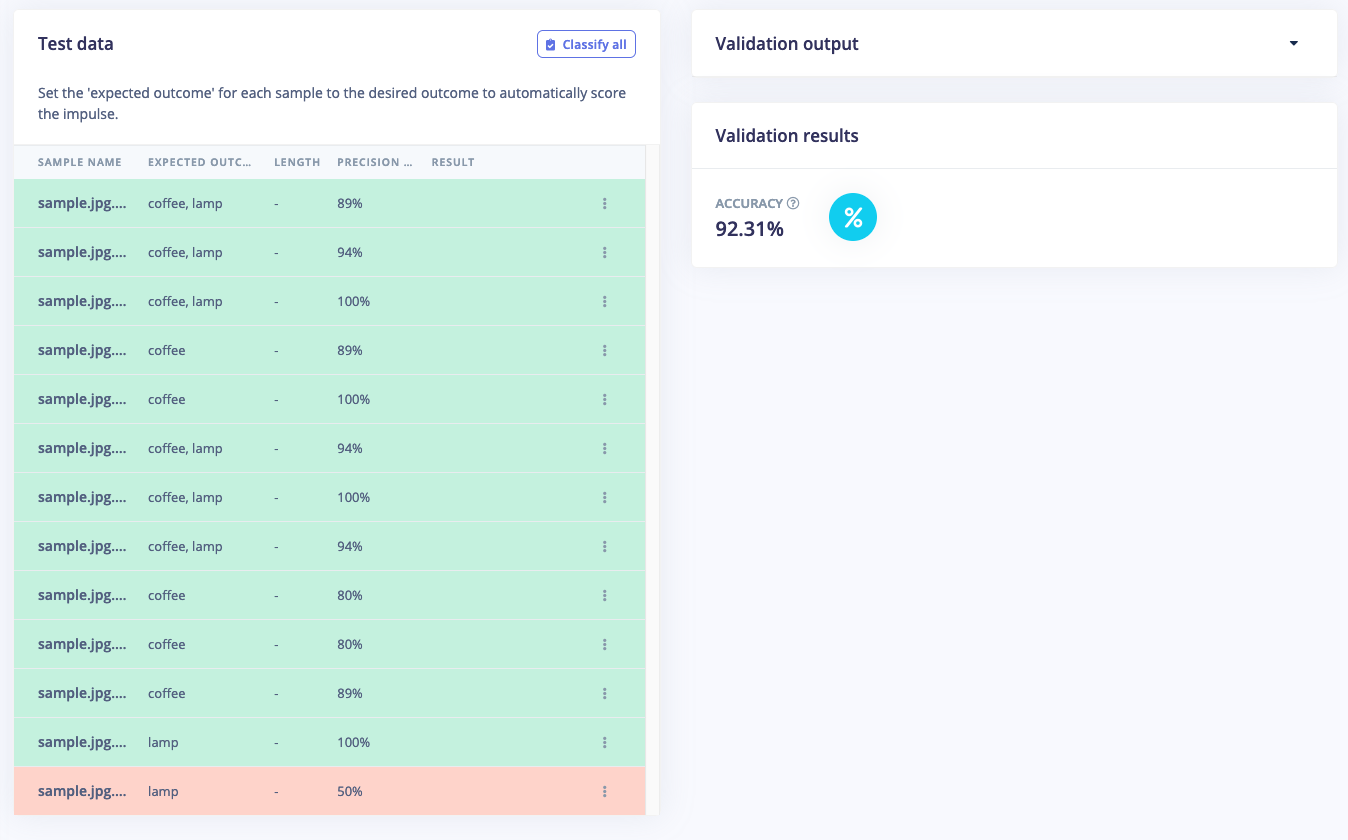
To see a classification in detail, click the three dots next to an item, and select Show classification. This brings you to the Live classification screen with much more details on the file (you can also capture new data directly from your development board from here). This screen can help you determine why items were misclassified.

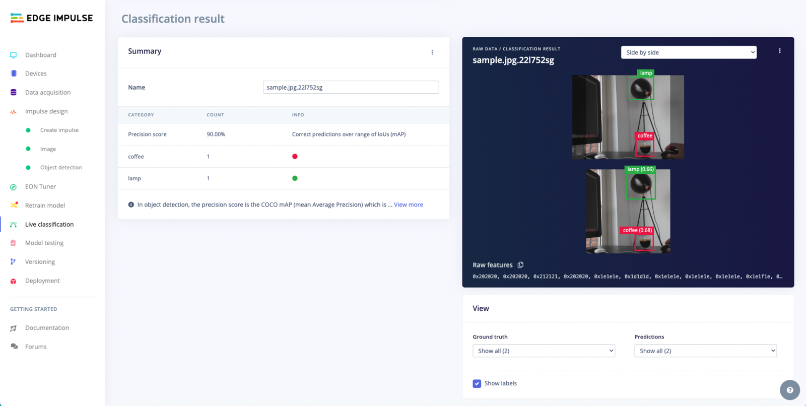
Live Classification Result

Live classification helps you determine how well your model works, showing the objects detected and the confidence score side by side.

This view is particularly useful for a direct comparison between the raw image and the model's interpretation. Each object detected in the image is highlighted with a bounding box. Alongside these boxes, you'll find labels and confidence scores, indicating what the model thinks each object is and how sure it is about its prediction. This mode is ideal for understanding the model's performance in terms of object localization and classification accuracy.

Overlay Mode for the Live Classification Result
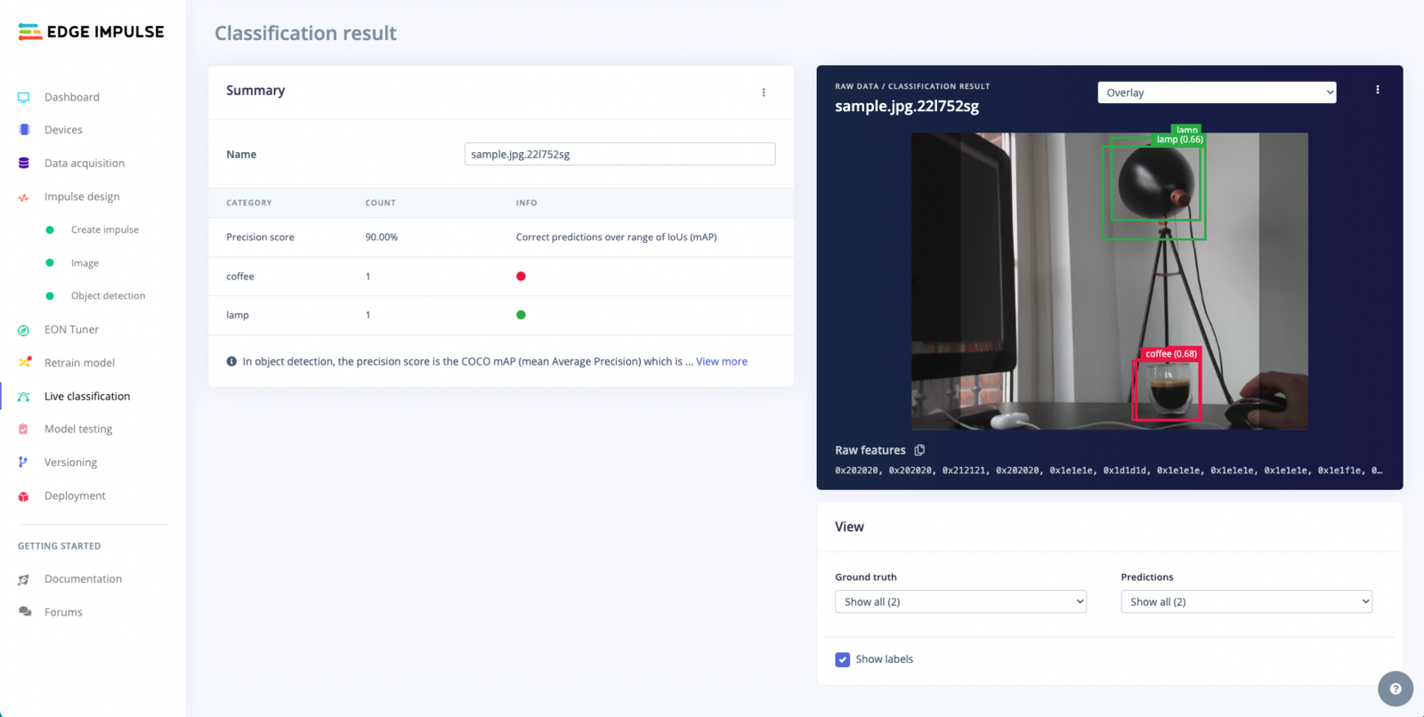
Changing to overlay mode provides a more integrated view by superimposing the model's detections directly onto the original image

In this view, bounding boxes are drawn around the detected objects, with labels and confidence scores displayed within the image context. This approach offers a clearer view of how the bounding boxes align with the objects in the image, making it easier to assess the precision of object localization. The overlay view is particularly useful for examining the model's ability to accurately detect and outline objects within a complex visual scene.

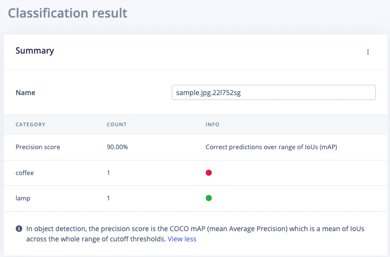
Summary Table

This table provides a concise summary of the performance metrics for an object detection model, using a specific sample file. The layout and contents are as follows.

Name: This field displays the name of the sample file analyzed by the model. For instance, 'sample.jpg.22l74u4f' is the file name in this case.

CATEGORY: Lists the types of objects that the model has been trained to detect. In this example, two categories are shown: 'coffee' and 'lamp'.

COUNT: Indicates the number of times each category was detected in the sample file. In this case, both 'coffee' and 'lamp' have a count of 1, meaning each object was detected once in the sample.

INFO: This column provides additional information about the model's performance. It displays the 'Precision score', which, in this example, is 95.00%. The precision score represents the model's accuracy in making correct predictions over a range of Intersection over Union (IoU) values, known as the mean Average Precision (mAP).

5. Running the model on your device

With the impulse designed, trained and verified you can deploy this model back to your device. This makes the model run without an internet connection, minimizes latency, and runs with minimum power consumption. Edge Impulse can package up the complete impulse - including the preprocessing steps, neural network weights, and classification code - in a single C++ library or model file that you can include in your embedded software.

Running the impulse on your Raspberry Pi 4 or Jetson Nano

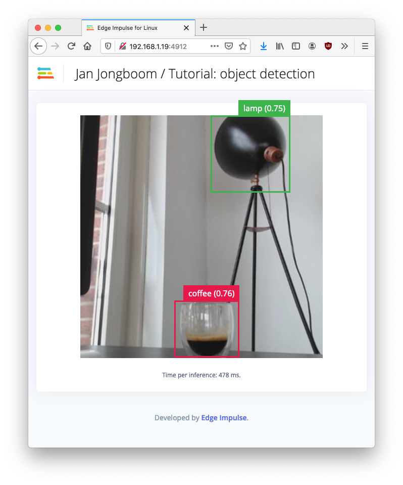
From the terminal just run edge-impulse-linux-runner. This will build and download your model, and then run it on your development board. If you're on the same network you can get a view of the camera, and the classification results directly from your dev board. You'll see a line like:

Want to see a feed of the camera and live classification in your browser? Go to http://192.168.1.19:4912

Open this URL in a browser to see your impulse running!

Object detection model running on a Raspberry Pi 4

Running the impulse on your mobile phone

On your mobile phone just click Switch to classification mode at the bottom of your phone screen. Point it at an object and press 'Capture'.

Integrating the model in your own application

Congratulations! You've added object detection to your sensors. Now that you've trained your model you can integrate your impulse in the firmware of your own edge device, see the Edge Impulse for Linux documentation for the Node.js, Python, Go and C++ SDKs that let you do this in a few lines of code and make this model run on any device. Here's an example of sending a text message through Twilio when an object is seen.

Or if you're interested in more, see our tutorials on Continuous motion recognition or Recognize sounds from audio. If you have a great idea for a different project, that's fine too. Edge Impulse lets you capture data from any sensor, build custom processing blocks to extract features, and you have full flexibility in your Machine Learning pipeline with the learning blocks.

We can't wait to see what you'll build! 🚀

Last updated