1. Prerequisites
For this tutorial you’ll need the:- Particle Photon2 Board with the Edge ML Kit.
2. Collecting your first data
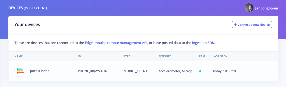
To build this project, you’ll need to collect some audio data that will be used to train the machine learning model. Since the goal is to detect the sound of a doorbell, you’ll need to collect some examples of that. You’ll also need some examples of typical background noise that doesn’t contain the sound of a doorbell, so the model can learn to discriminate between the two. These two types of examples represent the two classes we’ll be training our model to detect: unknown noise, or doorbell. Your phone will show up like any other device in Edge Impulse, and will automatically ask permission to use sensors. Let’s start by recording an example of background noise that doesn’t contain the sound of a doorbell. On your cell set the label tounknown, the sample length to 2 seconds. This indicates that you want to record 1 second of audio, and label the recorded data as unknown. You can later edit these labels if needed.
After you click Start recording, the device will capture a second of audio and transmit it to Edge Impulse.
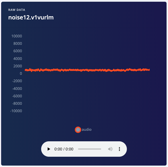
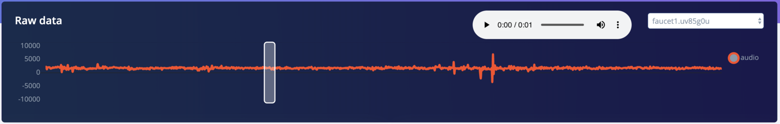
When the data has been uploaded, you will see a new line appear under ‘Collected data’ in the Data acquisition tab of your Edge Impulse project. You will also see the waveform of the audio in the ‘RAW DATA’ box. You can use the controls underneath to listen to the audio that was captured.
- doorbell - Record yourself ringing the doorbell in the same room
- unknown - Record the background noise in your house
3. Designing an impulse
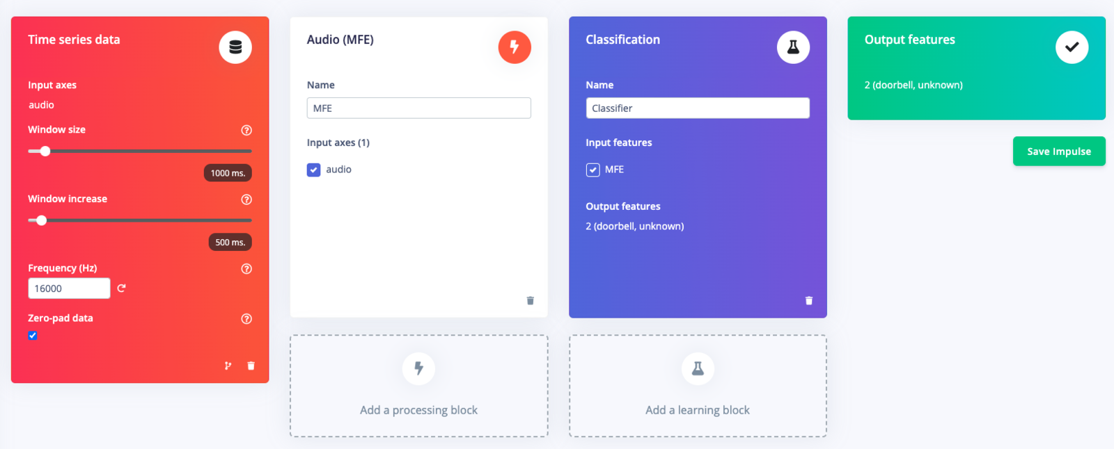
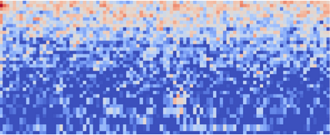
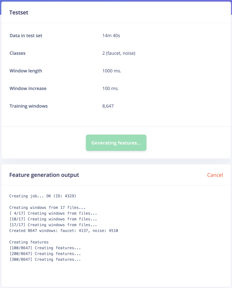
With the training set in place you can design an impulse. An impulse takes the raw data, slices it up in smaller windows, uses signal processing blocks to extract features, and then uses a learning block to classify new data. Signal processing blocks always return the same values for the same input and are used to make raw data easier to process, while learning blocks learn from past experiences. For this tutorial we’ll use the signal processing block. Then we’ll use a ‘Neural Network’ learning block, that takes these generated features and learns to distinguish between our different classes (circular or not). In the studio go to Create impulse, set the window size to1000 (you can click on the 1000 ms. text to enter an exact value), the window increase to 500, and add the ‘Audio MFCC’ and ‘Classification (Keras)’ blocks. Then click Save impulse.
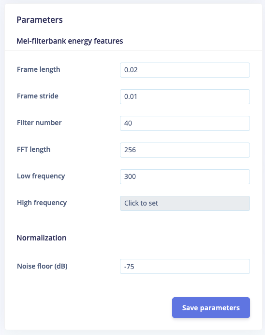
Configuring the MFCC block
Now that we’ve assembled the building blocks of our Impulse, we can configure each individual part. Click on the MFCC tab in the left hand navigation menu. You’ll see a page that looks like this: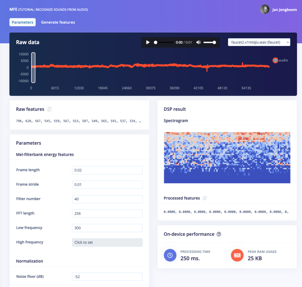
Configuring the neural network
With all data processed it’s time to start training a neural network. Neural networks are algorithms, modeled loosely after the human brain, that can learn to recognize patterns that appear in their training data. The network that we’re training here will take the MFCC as an input, and try to map this to one of two classes—doorbell or unknown. Click on NN Classifier in the left hand menu. You’ll see the following page: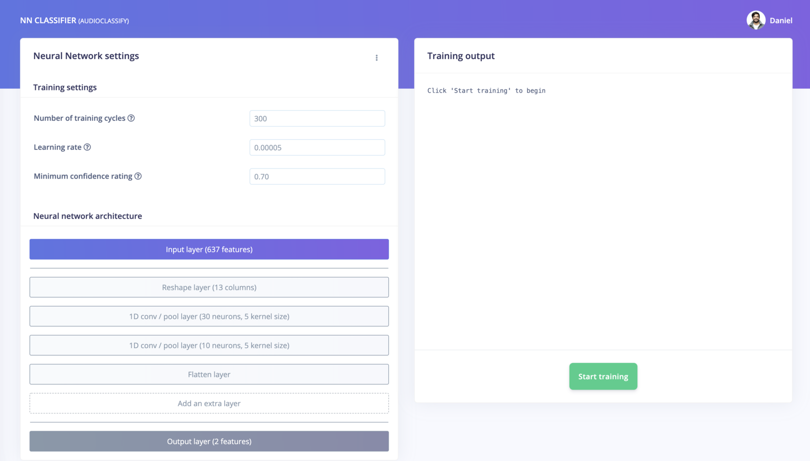
4. Classifying new data
The performance numbers in the previous step show that our model is working well on its training data, but it’s extremely important that we test the model on new, unseen data before deploying it in the real world. This will help us ensure the model has not learned to overfit the training data, which is a common occurrence. Edge Impulse provides some helpful tools for testing our model, including a way to capture live data from your device and immediately attempt to classify it. To try it out, click on Live classification in the left hand menu. Your device should show up in the ‘Classify new data’ panel. Capture 5 seconds of background noise by clicking Start sampling. The sample will be captured, uploaded, and classified. Once this has happened, you’ll see a breakdown of the results. Once the sample is uploaded, it is split into windows–in this case, a total of 41. These windows are then classified. As you can see, our model classified all 41 windows of the captured audio as noise. This is a great result! Our model has correctly identified that the audio was background noise, even though this is new data that was not part of its training set. Of course, it’s possible some of the windows may be classified incorrectly. If your model didn’t perform perfectly, don’t worry. We’ll get to troubleshooting later.5. Model testing
Using the Live classification tab, you can easily try out your model and get an idea of how it performs. But to be really sure that it is working well, we need to do some more rigorous testing. That’s where the Model testing tab comes in. If you open it up, you’ll see the sample we just captured listed in the Test data panel. In addition to its training data, every Edge Impulse project also has a test dataset. Samples captured in Live classification are automatically saved to the test dataset, and the Model testing tab lists all of the test data. To use the sample we’ve just captured for testing, we should correctly set its expected outcome. Click the⋮ icon and select Edit expected outcome, then enter noise. Now, select the sample using the checkbox to the left of the table and click Classify selected.
You’ll see that the model’s accuracy has been rated based on the test data. Right now, this doesn’t give us much more information that just classifying the same sample in the Live classification tab. But if you build up a big, comprehensive set of test samples, you can use the Model testing tab to measure how your model is performing on real data.
Ideally, you’ll want to collect a test set that contains a minimum of 25% the amount of data of your training set. So, if you’ve collected 10 minutes of training data, you should collect at least 2.5 minutes of test data. You should make sure this test data represents a wide range of possible conditions, so that it evaluates how the model performs with many different types of inputs. For example, collecting test audio for several different doorbells, perhaps moving collecting the audio in a different room, is a good idea.
You can use the Data acquisition tab to manage your test data. Open the tab, and then click Test data at the top. Then, use the Record new data panel to capture a few minutes of test data, including audio for both background noise and doorbells. Make sure the samples are labelled correctly. Once you’re done, head back to the Model testing tab, select all the samples, and click Classify selected.
The screenshot shows classification results from a large number of test samples (there are more on the page than would fit in the screenshot). It’s normal for a model to perform less well on entirely fresh data.
For each test sample, the panel shows a breakdown of its individual performance. Samples that contain a lot of misclassifications are valuable, since they have examples of types of audio that our model does not fit. It’s often worth adding these to your training data, which you can do by clicking the ⋮ icon and selecting Move to training set. If you do this, you should add some new test data to make up for the loss!
Testing your model helps confirm that it works in real life, and it’s something you should do after every change. However, if you often make tweaks to your model to try to improve its performance on the test dataset, your model may gradually start to overfit to the test dataset, and it will lose its value as a metric. To avoid this, continually add fresh data to your test dataset.
Data hygieneIt’s extremely important that data is never duplicated between your training and test datasets. Your model will naturally perform well on the data that it was trained on, so if there are duplicate samples then your test results will indicate better performance than your model will achieve in the real world.
6. Model troubleshooting
If the network performed well, great! But what if it performed poorly? There could be a variety of reasons, but the most common ones are:- The data does not look like other data the network has seen before. This is common when someone uses the device in a way that you didn’t add to the test set. You can add the current file to the test set by adding the correct label in the ‘Expected outcome’ field, clicking
⋮, then selecting Move to training set. - The model has not been trained enough. Increase number of epochs to
200and see if performance increases (the classified file is stored, and you can load it through ‘Classify existing validation sample’). - The model is overfitting and thus performs poorly on new data. Try reducing the number of epochs, reducing the learning rate, or adding more data.
- The neural network architecture is not a great fit for your data. Play with the number of layers and neurons and see if performance improves.
7. Deploying to your device
With the impulse designed, trained and verified you can deploy this model back to your device. This makes the model run without an internet connection, minimizes latency, and runs with minimum power consumption. To export your model, click on Deployment in the menu. Then under ‘Build firmware’ select the Particle Library.8. Flashing the device
Once optimized parameters have been found, you can click Build. This will build a particle workbench compatible package that will run on your development board. After building is completed you’ll get prompted to download a zipfile. Save this on your computer. A pop-up video will show how the download process works. After unzipping the downloaded file, you can open the project in Particle Workbench.Flash a Particle Photon 2 Project
The development board does not come with the Edge Impulse firmware. To flash the Edge Impulse firmware:- Open a new VS Code window, ensure that Particle Workbench has been installed (see above)
- Use VS Code Command Palette and type in Particle: Import Project
- Select the
project.propertiesfile in the directory that you just downloaded and extracted from the section above.
- Select the
- Use VS Code Command Palette and type in Particle: Configure Project for Device
- Select
deviceOS@5.3.2(or a later version) - Choose a target. (e.g. P2 , this option is also used for the Photon 2).
- Select
- It is sometimes needed to manually put your Device into DFU Mode. You may proceed to the next step, but if you get an error indicating that “No DFU capable USB device available” then please follow these step.
- Hold down both the RESET and MODE buttons.
- Release only the RESET button, while holding the MODE button.
- Wait for the LED to start flashing yellow.
- Release the MODE button.
- Compile and Flash in one command with: Particle: Flash application & DeviceOS (local)
Serial Connection to Computer
The Particle libraries generated by Edge Impulse have serial output through a virtual COM port on the serial cable. The serial settings are 115200, 8, N, 1. Particle Workbench contains a serial monitor accessible via Particle: Serial Monitor via the VS Code Command Palette.Device compatibilityInitial release of the particle integration will rely on the particle-ingestion project and the data forwarder to be installed on the device and computer. This is only tested on the Particle Photon 2, but should run on other devices as well.
Stand Alone Example with Static Buffer
This standalone example project contains minimal code required to run the imported impulse on the device. This code is located inmain.cpp. In this minimal code example, inference is run from a static buffer of input feature data. To verify that our embedded model achieves the exact same results as the model trained in Studio, we want to copy the same input features from Studio into the static buffer in main.cpp.
To do this, first head back to Edge Impulse Studio and click on the Live classification tab. Follow this video for instructions.
In
main.cpp paste the raw features inside the static const float features[] definition, for example:
main.cpp to run classification on live data.
Running the model on the device
Follow the flashing instructions above to run on device. Victory! You’ve now built your first on-device machine learning model.