Continuous inference modeContinuous inferencing is automatically enabled for any impulses that use audio. Build and flash a ready-to-go binary for your development board from the Deployment tab in the studio, then - from a command prompt or terminal window - run
edge-impulse-run-impulse --continuous.An Arduino sketch that demonstrates continuous audio sampling is part of the Arduino library deployment option. After importing the library into the Arduino IDE, look under ‘Examples’ for ‘nano_ble33_sense_audio_continuous’.Continuous Inferencing
In the normal (non-continuous) inference mode when classifying data you sample data until you have a full window of data (e.g. 1 second for a keyword spotting model, see the Create impulse tab in the studio), you then classify this window (using therun_classifier function), and a prediction is returned. Then you empty the buffer, sample new data, and run the inferencing again. Naturally this has some caveats when deploying your model in the real world: 1) you have a delay between windows, as classifying the window takes some time and you’re not sampling then, making it possible to miss events. 2) there’s no overlap between windows, thus if an event is at the very end of the window, not the full event might be captured - leading to a wrong classification.
To mitigate this we have added several new features to the Edge Impulse SDK.
1. Model slices
Using continuous inferencing, smaller sampling buffers (slices) are used and passed to the inferencing process. In the inferencing process, the buffers are time sequentially placed in a FIFO (First In First Out) buffer that matches the model size. After each iteration, the oldest slice is removed at the end of the buffer and a new slice is inserted at the beginning. On each slice now, the inference is run multiple times (depending on the number of slices used for a model). For example, a 1-second keyword model with 4 slices (each 250 ms), will infer each slice 4 times. So if now the keyword is on 2 edges of the slice buffers, they’re glued back together in the FIFO buffer and the keyword will be classified correctly.2. Averaging
Another advantage of this technique is that it filters out false positives. Take for instance a yes-no keyword spotting model. The word ‘yesterday’ should not be classified as a yes (or no). But if the ‘yes-’ is sampled in the first buffer and ‘-terday’ in the next, there is a big chance that the inference step will classify the first buffer as a yes. By running inference multiple times over the slices, continuous inferencing will filter out this false positive. When the ‘yes’ buffer enters the FIFO it will surely classify as a ‘yes’. But as the rest of the word enters, the classified value for ‘yes’ will drop quickly. We just have to make sure that we don’t react on peak values. Therefore a moving average filter averages the classified output and so flattens the peaks. To have a valid ‘yes’, we now need multiple high-rated classifications.Continuous audio sampling
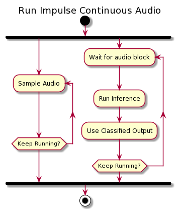
In the standard way of running the impulse, the steps of collecting data and running the inference are run sequentially. First, the audio is sampled, filling a block the size of the model. This block is sent to the inferencing part, where first the features are extracted and then the inference is run. Finally, the classified output is used in your application (by default the output will be printed over the serial connection).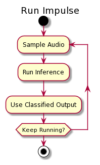
Implementing continuous audio sampling
We’ve implemented continuous audio sampling already on the ST B-L475E-IOT01A and the Arduino Nano 33 BLE Sense targets (the firmware for both targets is open source), but here’s a guideline to implementing this on your own targets.Prerequisites
The embedded target needs to support running of multiple processes in parallel. This can either be achieved by an operating system; 1 low priority thread will run inferencing and 1 high priority thread will collect sample data. Or the processor should support processor offloading. This is usually done by the audio peripheral or DMA (Direct Memory Access). Here audio samples are collected in a buffer without involvement of the processor.Double buffering
How do we know when new sample data is available? For this we use a double buffering mechanism. Hereby 2 sample buffers are used:- 1 buffer for the audio sampling process, filling the buffer with new sample data
- 1 buffer for the inference process, get sample data out the buffer, extract the features and run inference
Timing and memory is everything
There are 2 constraints in this story: timing and memory. When switching the buffers there must be a 100% guarantee that the inference process is finished when the sampling process passes a full buffer. If not, the sampling process overruns the buffer and sampled data will get lost. When that happens on the ST B-L475E-IOT01A or the Arduino Nano 33 BLE Sense target, running the impulse is aborted and the following error is returned:EI_CLASSIFIER_SLICES_PER_MODEL_WINDOW macro is used to set the number of slices to fill the complete model window. The more slices per model, the smaller the slice size, thereby the more inference cycles on the sampled data. Leading to more accurate results. The sampling process uses this macro for the buffer size. Where following rule applies: the bigger the buffer, the longer the sampling cycle. So on targets with lower processing capabilities, we can increase this macro to meet the timing constraint.
Increasing the slice size, increases the volatile memory uses times 2 (since we use double buffering). On a target with limited volatile memory this could be a problem. In this case you want the slice size to be small.
Double buffering in action
On both the ST B-L475E-IOT01A and Arduino Nano 33 BLE Sense targets the audio sampling process calls theaudio_buffer_inference_callback() function when there is data. Here the number of samples (inference.n_samples) are stored in one of the buffers. When the buffer is full, the buffers are switched by toggling inference.buf_select. The inference process is signaled by setting the flag inference.buf_ready.
signal_t structure to reference the selected buffer: