FOMO: Object detection for constrained devices

Edge Impulse FOMO (Faster Objects, More Objects) is a novel machine learning algorithm that brings object detection to highly constrained devices. It lets you count objects, find the location of objects in an image, and track multiple objects in real-time using up to 30x less processing power and memory than MobileNet SSD or YOLOv5.

Tutorials

Want to see FOMO in action? Check out our Detect objects with centroids (FOMO) tutorial.

For example, FOMO lets you do 60 fps object detection on a Raspberry Pi 4:

And here's FOMO doing 30 fps object detection on an Arduino Nicla Vision (Cortex-M7 MCU), using 245K RAM.

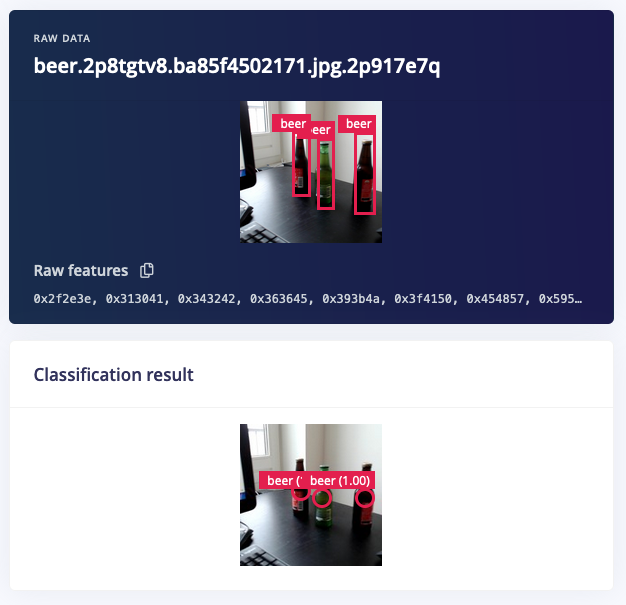
You can find the complete Edge Impulse project with the beers vs. cans model, including all data and configuration here: https://studio.edgeimpulse.com/public/89078/latest.

How does this 🪄 work?

So how does that work? First, a small primer. Let's say you want to detect whether you see a face in front of your sensor. You can approach this in two ways. You can train a simple binary classifier, which says either "face" or "no face", or you can train a complex object detection model which tells you "I see a face at this x, y point and of this size". Object detection is thus great when you need to know the exact location of something, or if you want to count multiple things (the simple classifier cannot do that) - but it's computationally much more intensive, and you typically need much more data for it.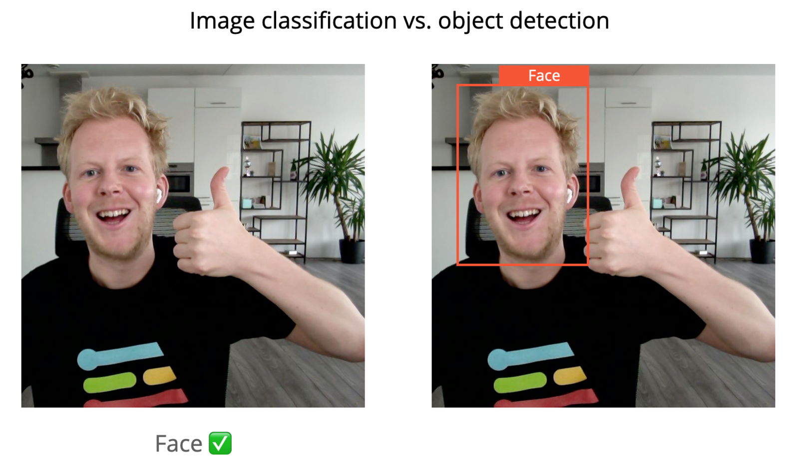

Image classification vs object detection

The design goal for FOMO was to get the best of both worlds: the computational power required for simple image classification, but with the additional information on location and object count that object detection gives us.

Heat maps

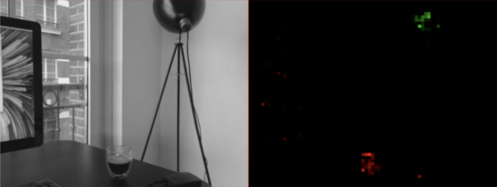
The first thing to realize is that while the output of the image classifier is "face" / "no face" (and thus no locality is preserved in the outcome) the underlying neural network architecture consists of a number of convolutional layers. A way to think about these layers is that every layer creates a diffused lower-resolution image of the previous layer. E.g. if you have a 16x16 image the width/height of the layers may be:

1. 16x16

2. 4x4

3. 1x1

Each 'pixel' in the second layer maps roughly to a 4x4 block of pixels in the input layer, and the interesting part is that locality is somewhat preserved. The 'pixel' in layer 2 at (0, 0) will roughly map back to the top left corner of the input image. The deeper you go in a normal image classification network, the less of this locality (or "receptive field") is preserved until you finally have just 1 outcome.

FOMO uses the same architecture, but cuts off the last layers of a standard image classification model and replaces this layer with a per-region class probability map (e.g. a 4x4 map in the example above). It then has a custom loss function which forces the network to fully preserve the locality in the final layer. This essentially gives you a heatmap of where the objects are.

From input image to heat map (cup in red, lamp in green)

The resolution of the heat map is determined by where you cut off the layers of the network. For the FOMO model trained above (on the beer bottles) we do this when the size of the heat map is 8x smaller than the input image (input image of 160x160 will yield a 20x20 heat map), but this is configurable. When you set this to 1:1 this actually gives you pixel-level segmentation and the ability to count a lot of small objects.

Here's a former iteration of the FOMO approach used to count individual bees (heat map 2x smaller than the input size).

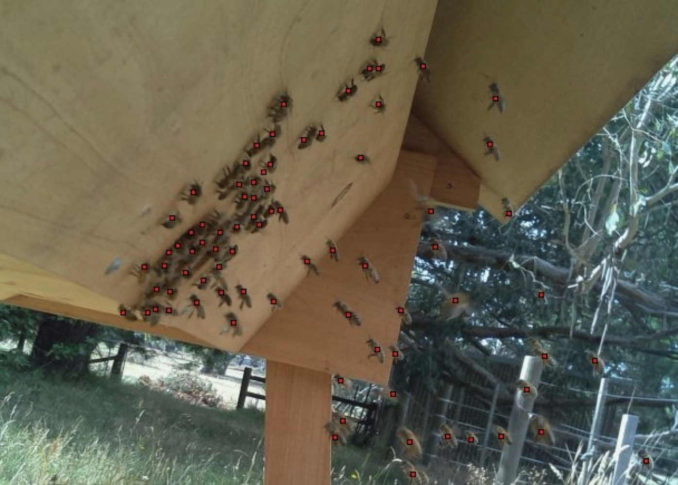
Training on centroids

A difference between FOMO and other object detection algorithms is that it does not output bounding boxes, but it's easy to go from heat map to bounding boxes. Just draw a box around a highlighted area.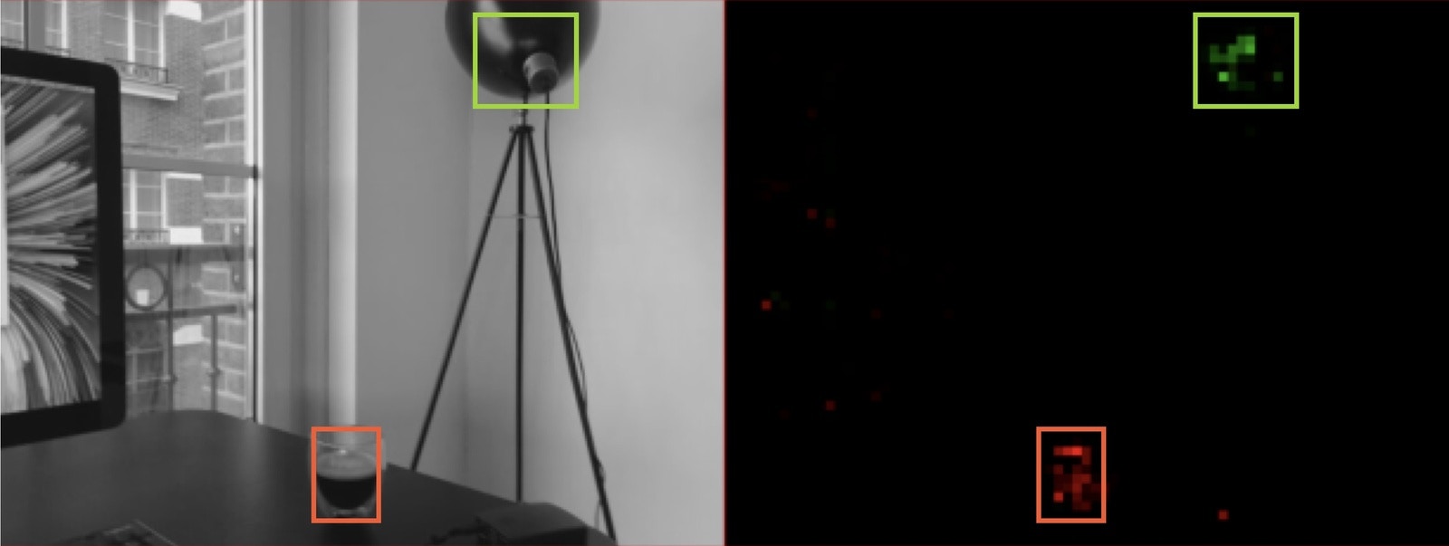

From heat map to bounding boxes

However, when working with early customers we realized that bounding boxes are merely an implementation detail of other object detection networks, and are not a typical requirement. Very often the size of objects is not important as cameras are in fixed locations (and objects thus fixed size), but rather you just want the location and the count of objects.

Thus, we now train on the centroids of objects. This makes it much easier to count objects that are close (every activation in the heat map is an object), and the convolutional nature of the neural network ensures we look around the centroid for the object anyway.

Training on the centroids of beer bottles. On top the source labels, at the bottom the inference result.

A downside of the heat map is that each cell acts as its own classifier. E.g. if your classes are "lamp", "plant" and "background" each cell will be either lamp, plant, or background. It's thus not possible to detect objects with overlapping centroids. You can see this in the Raspberry Pi 4 video above at 00:18 where the beer bottles are too close together. This can be solved by using a higher resolution heat map.

Flexible and very, very fast

A really cool benefit of FOMO is that it's fully convolutional. If you set an image:heat map factor of 8 you can throw in a 96x96 image (outputs 12x12 heat map), a 320x320 image (outputs 40x40 heat map), or even a 1024x1024 image (outputs 128x128 heat map). This makes FOMO incredibly flexible, and useful even if you have very large images that need to be analyzed (e.g. in fault detection where the faults might be very, very small). You can even train on smaller patches, and then scale up during inference.

Additionally FOMO is compatible with any MobileNetV2 model. Depending on where the model needs to run you can pick a model with a higher or lower alpha, and transfer learning also works (although you need to train your base models specifically with FOMO in mind). This makes it easy for end customers to use their existing models and fine-tune them with FOMO to also add locality (e.g. we have customers with large transfer learning models for wildlife detection).

Together this gives FOMO the capabilities to scale from the smallest microcontrollers all the way to full gateways or GPUs. Just some numbers:

1. The video on the top classifies 60 times / second on a stock Raspberry Pi 4 (160x160 grayscale input, MobileNetV2 0.1 alpha). This is 20x faster than MobileNet SSD which does ~3 frames/second.

2. The second video on the top classifies 30 times / second on an Arduino Nicla Vision board with a Cortex-M7 MCU running at 480MHz) in ~240K of RAM (96x96 grayscale input, MobileNetV2 0.35 alpha).

3. During Edge Impulse Imagine we demonstrated a FOMO model running on a Himax WE-I Plus doing 14 frames per second on a DSP (video). This model ran in under 150KB of RAM (96x96 grayscale input, MobileNetV2 0.1 alpha). [1]

4. The smallest version of FOMO (96x96 grayscale input, MobileNetV2 0.1 alpha) runs in <100KB RAM and ~10 fps. on a Cortex-M4F at 80MHz. [1]

[1] Models compiled using EON Compiler.

How to get started?

To build your first FOMO models:

1. Create a new project in Edge Impulse.

2. Make sure to set your labeling method to 'Bounding boxes (object detection)'.

3. Collect and prepare your dataset as in object detection.

4. Add an 'Object Detection (Images)' block to your impulse.

5. Under Images, select 'Grayscale'

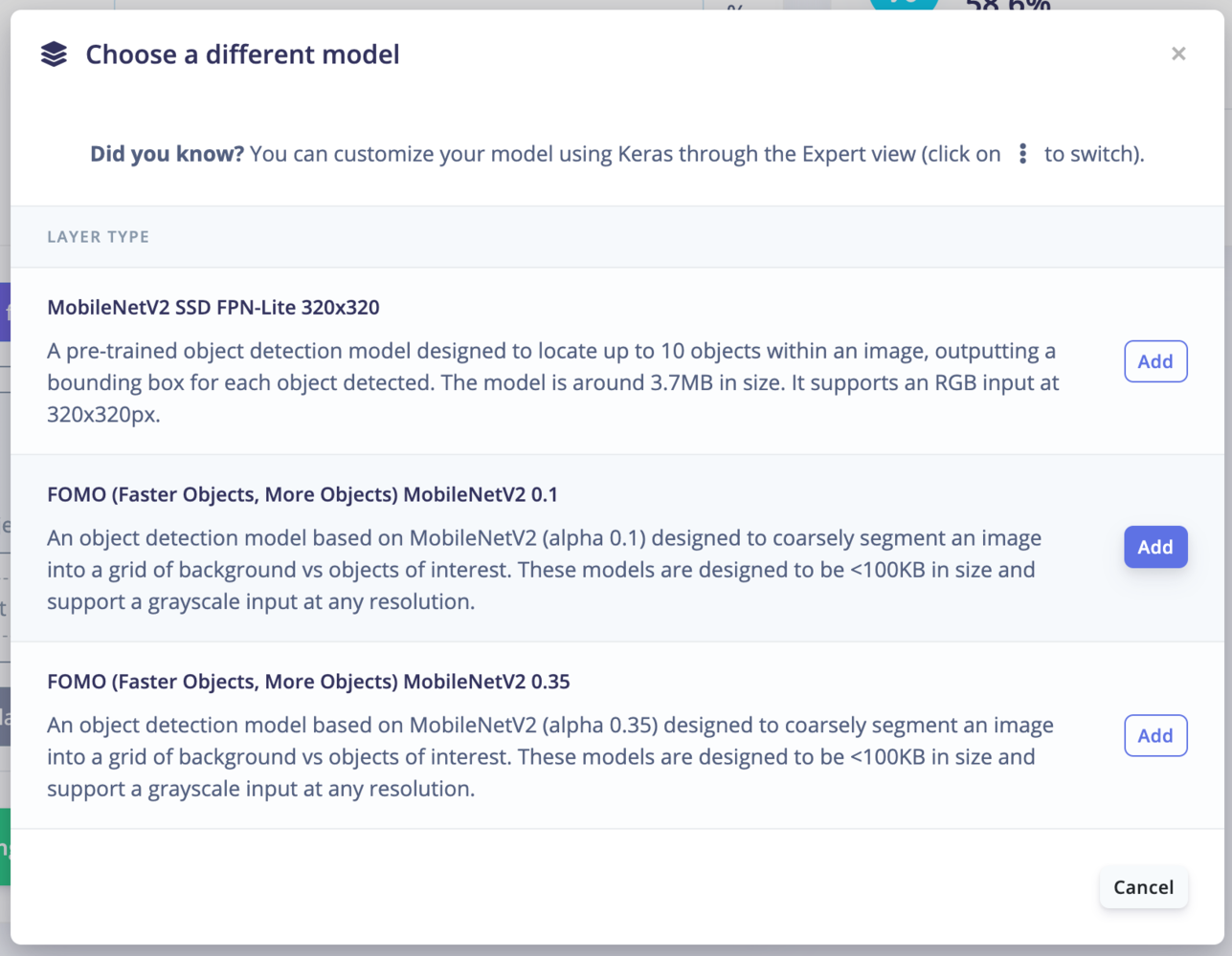
6. Under Object detection, select 'Choose a different model' and select one of the FOMO models.

7. Make sure to lower the learning rate to 0.001 to start.

Selecting a FOMO model in Edge Impulse

FOMO is currently compatible with all fully-supported development boards that have a camera, and with Edge Impulse for Linux (any client). Of course, you can export your model as a C++ Library and integrate it as usual on any device or development board, the output format of models is compatible with normal object detection models; and our SDK runs on almost anything under the sun (see Running your impulse locally for an overview) from RTOS's to bare-metal to special accelerators and GPUs.

Expert mode tips

Additional configuration for FOMO can be accessed via expert mode.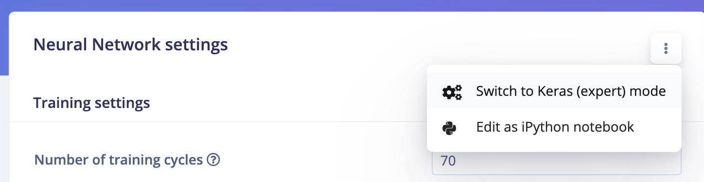

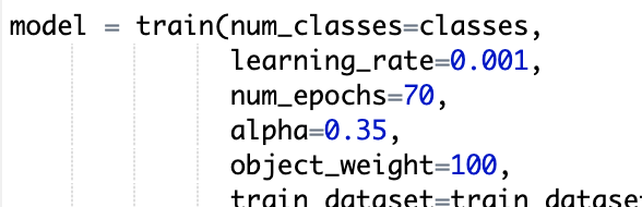
Accessing expert mode

Object weighting

FOMO is sensitive to the ratio of objects to background cells in the labelled data. By default the configuration is to weight object output cells x100 in the loss function, object_weight=100, as a way of balancing what is usually a majority of background. This value was chosen as a sweet spot for a number of example use cases. In scenarios where the objects to detect are relatively rare this value can be increased, e.g. to 1000, to have the model focus even more on object detection (at the expense of potentially more false detections).

MobileNet cut point

FOMO uses MobileNetV2 as a base model for its trunk and by default does a spatial reduction of 1/8th from input to output (e.g. a 96x96 input results in a 12x12 output). This is implemented by cutting MobileNet off at the intermediate layer block_6_expand_relu

MobileNetV2 cut point

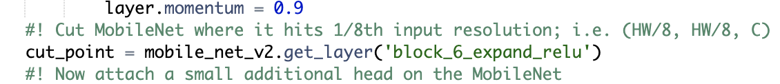
Choosing a different cut_point results in a different spatial reduction; e.g. if we cut higher at block_3_expand_relu FOMO will instead only do a spatial reduction of 1/4 (i.e. a 96x96 input results in a 24x24output)

Note though; this means taking much less of the MobileNet backbone and results in a model with only 1/2 the params. Switching to a higher alpha may counteract this parameter reduction. Later FOMO releases will counter this parameter reduction with a UNet style architecture.

FOMO classifier capacity

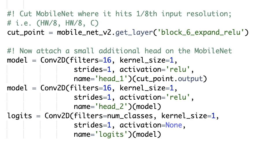
FOMO can be thought of logically as the first section of MobileNetV2 followed by a standard classifier where the classifier is applied in a fully convolutional fashion.

In the default configuration this FOMO classifier is equivalent to a single dense layer with 32 nodes followed by a classifier with num_classes outputs.

FOMO uses a convolutional classifier.

For a three way classifier, using the default cut point, the result is a classifier head with ~3200 parameters.

 LAYER                          SHAPE                NUMBER OF PARAMETERS
 block_6_expand_relu (ReLU)     (None, 20, 20, 96)   0
 head (Conv2D)                  (None, 20, 20, 32)   3104
 logits (Conv2D)                (None, 20, 20, 3)    99

We have the option of increasing the capacity of this classifier head by either 1) increasing the number of filters in the Conv2D layer, 2) adding additional layers or 3) doing both.

For example we might change the number of filters from 32 to 16, as well as adding another convolutional layer, as follows.

Adding an additional layer to the classifier of FOMO

 LAYER                          SHAPE                NUMBER OF PARAMETERS
 block_6_expand_relu (ReLU)     (None, 20, 20, 96)   0
 head_1 (Conv2D)                (None, 20, 20, 16)   1552
 head_2 (Conv2D)                (None, 20, 20, 16)   272
 logits (Conv2D)                (None, 20, 20, 3)    51

For some problems an additional layer can improve performance, and in this case actually uses less parameters. It can though potentially take longer to train and require more data. In future releases the tuning of this aspect of FOMO can be handled by the EON Tuner.

Performance and Minimum Requirements

Just like the rest of our Neural Network-based learning blocks, FOMO is delivered as a set of basic math routines free of runtime dependencies. This means that there are virtually no limitations to running FOMO, other than:

1. Making sure the model itself can fit into the target's memory (flash/RAM), and

2. making sure the target also has enough memory to hold the image buffer (flash/RAM)in addition to your application logic

In all, we have seen buffer, model and app logic (including wireless stack) fit in as little as 200KB for 64x64 pixel images. But we would definitely recommend a target with at least 512KB so that you can take advantage of larger image sizes and a wider range of model optimizations.

With regards to latency, the speed of the target will determine the maximum number of frames that can be processed in a given interval (fps). This will of course be influenced by any other tasks the CPU may need to complete, but we have consistently seen MCUs running @ 80MHz complete a full pass on a 64x64 pixel image in under one second, which should translate to just under 1fps once you add the rest of your app logic. Keep in mind that frame throughput can increase dramatically at higher speeds or when tensor acceleration is available. We have measured 40-60 fps consistently on a Raspberry Pi 4 and ~15 fps on unaccelerated 480MHz targets. The table below summarizes this trade-off:

Requirement	Minimum	Recommended
Memory Footprint (RAM)	256 KB 64x64 pixels (B&W, buffer included)	≥ 512 KB 96x96 pixels (B&W, buffer Included)
Latency (100% load)	80 MHz < 1 fps	> 80 MHz + acceleration ~15 fps @ 480MHz 40-60fps in RPi4