Visual anomaly detection (FOMO-AD)

Training visual anomaly detection (FOMO-AD) models involves developing algorithms to identify unusual patterns or anomalies in image data that do not conform to the expected behavior. These models are crucial in various applications, including industrial inspection, medical imaging, and logistics.

For visual anomaly detection use cases, i.e. handling defect identification in computer vision applications, Edge Impulse provides the Visual Anomaly Detection (previously the FOMO-AD block), based on a selectable backbone for feature extraction and a scoring function (PatchCore, GMM anomaly detection).

Neural networks are powerful but have a major drawback: handling unseen data, like defects in a product during manufacturing, is a challenge due to their reliance on existing training data. Even entirely novel inputs often get misclassified into existing categories.

Selectable scoring functions for Visual Anomaly Detection

Only available with Edge Impulse Enterprise Plan

Try our FREE Enterprise Trial today.

Scoring functions

PatchCore

PatchCore is an unsupervised method for detecting anomalies in images by focusing on small regions, called patches. It first learns what "normal" looks like by extracting features from patches of normal images using a pre-trained neural network. Instead of storing all normal patches, it creates a compact summary (core-set) of them to save memory.

When a new image is checked, PatchCore compares its patches to this core-set. If a patch significantly differs from the normal ones, it’s flagged as an anomaly. The system can also pinpoint where the anomaly is and assign a score to measure its severity. This approach is both memory-efficient and scalable, making it useful for real-time or large-scale tasks, without needing labeled data of anomalies in the training dataset.

Gaussian Mixture Model (GMM)

A Gaussian Mixture Model represents a probability distribution as a mixture of multiple Gaussian (normal) distributions. Each Gaussian component in the mixture represents a cluster of data points with similar characteristics. Thus, GMMs work using the assumption that the samples within a dataset can be modeled using different Gaussian distributions.

Anomaly detection using GMM involves identifying data points with low probabilities. If a data point has a significantly lower probability of being generated by the mixture model compared to most other data points, it is considered an anomaly; this will output a high anomaly score.

GMM has some overlap with K-means, however, K-means clusters are always circular, spherical or hyperspherical when GMM can model elliptical clusters.

Looking for another anomaly detection technique? Or are you using time-based frequency sensor data? See Anomaly detection (GMM) or Anomaly detection (K-Means)

How does GMM work?

1. During training, X number of Gaussian probability distributions are learned from the data where X is the number of components (or clusters) defined in the learning block page. Samples are assigned to one of the distributions based on the probability that it belongs to each. We use Sklearn under the hood and the anomaly score corresponds to the log-likelihood.

2. For the inference, we calculate the probability (which can be interpreted as a distance on a graph) for a new data point belonging to one of the populations in the training data. If the data point belongs to a cluster, the anomaly score will be low.

Setting up the Visual Anomaly Detection learning block

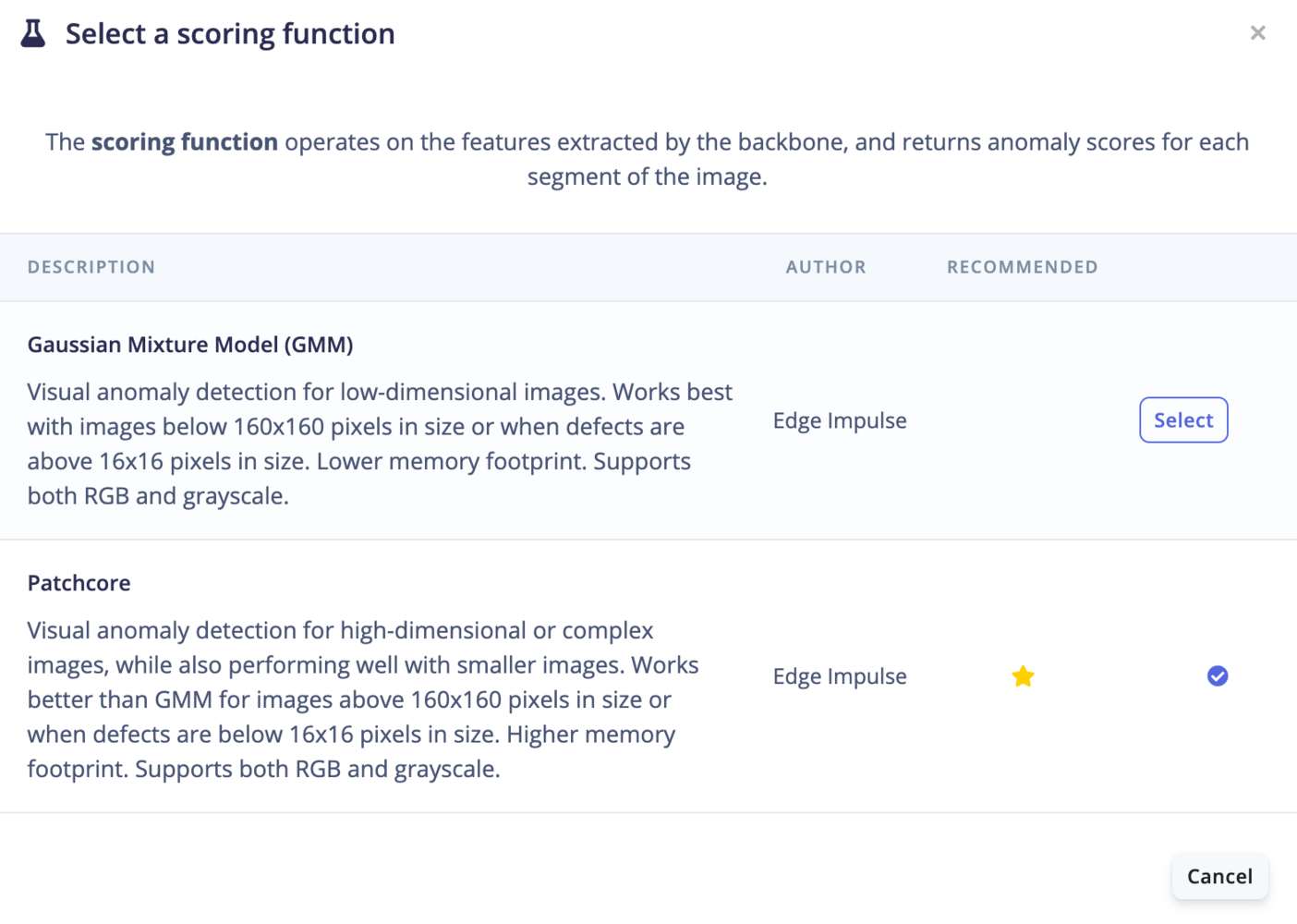
First, select your Scoring function and Backbone of choice under "Neural network architecture":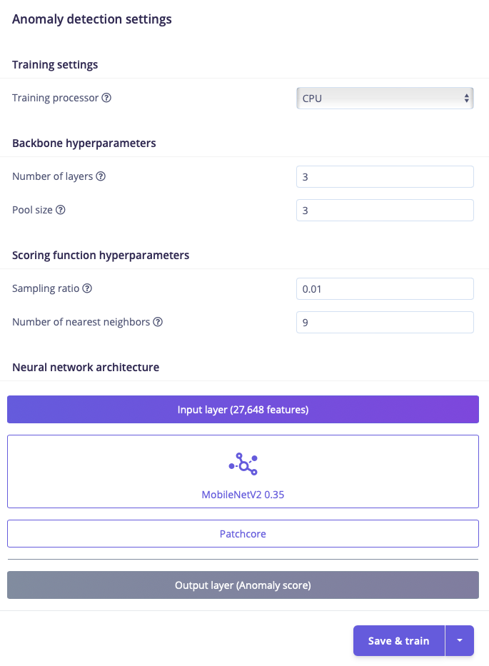

Settings for Visual Anomaly Detection

Based on the deployment target configuration of your project, the Visual Anomaly Detection (FOMO-AD) learning block will default to either GMM for a low-power device or Patchcore for a high-power device.

PatchCore

The PatchCore Visual Anomaly Detection learning block has multiple adjustable parameters. The neural network architecture is also adjustable.

• Number of layers: The number of layers in the feature extractor

  • Try with a single layer and then increase layers if the anomalies are not being detected.

• Pool size: The pool size for the feature extractor

  • The kernel size for average 2D pooling over the extracted features, size 1 = no pooling.

• Sampling ratio: The sampling ratio for the core set, used for anomaly scoring

  • This is the ratio of features from the training set patches that are saved to the memory bank to give an anomaly score to each patch at inference time. Larger values increases the size of the model and can lead to overfitting to the training data.

• Number of nearest neighbors: The number of nearest neighbors to consider, used for anomaly scoring

  • The number of nearest neighbors controls how many neighbors to compare patches to when calculating the anomaly score for each patch.

GMM

The GMM Visual Anomaly Detection learning block has one adjustable parameter: capacity. The neural network architecture is also adjustable.

Regardless of what resolution we intend to use for raw image input, we empirically get the best result for anomaly detection from using 96x96 ImageNet weights. We use 96x96 weights since we'll only being used the start of MobileNet to reduce to 1/8th input.

Capacity

The higher the capacity, the higher the number of (Gaussian) components, and the more adapted the model becomes to the original distribution.

Train

Click on Start training to trigger the learning process. Once trained you will obtain a trained model view that looks like the following: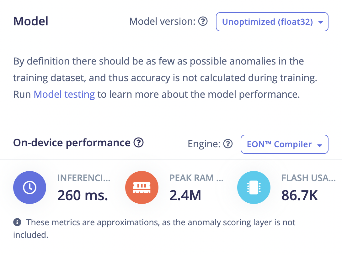

Trained model view for Visual Anomaly Detection.

Continue to the Model testing tab to see the performance results of your model.

Note: By definition, there should not be any anomalies in the training dataset, and thus accuracy is not calculated during training. Run Model testing to learn more about the model performance and to view per region anomalous scoring results.

Testing the Visual Anomaly Detection learning block

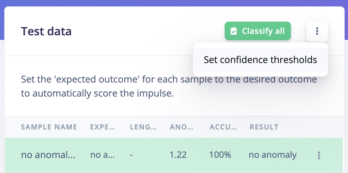
Navigate to the Model testing page and click on Classify all: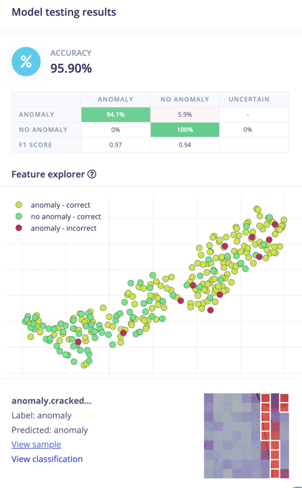

Model testing view with sample selected.

Limitation

Make sure to label your samples exactly as anomaly or no anomaly in your test dataset so they can be used in the F1 score calculation. We are working on making this more flexible.

Confidence threshold

In the example above, you will see that some samples have regions that are considered as no anomaly while the expected output is an anomaly. To adjust this prediction, you can set the Confidence thresholds, where you can also see the default or suggested value: "Suggested value is 16.6, based on the top anomaly scores in the training dataset.":

View confidence thresholds.

Set confidence thresholds.

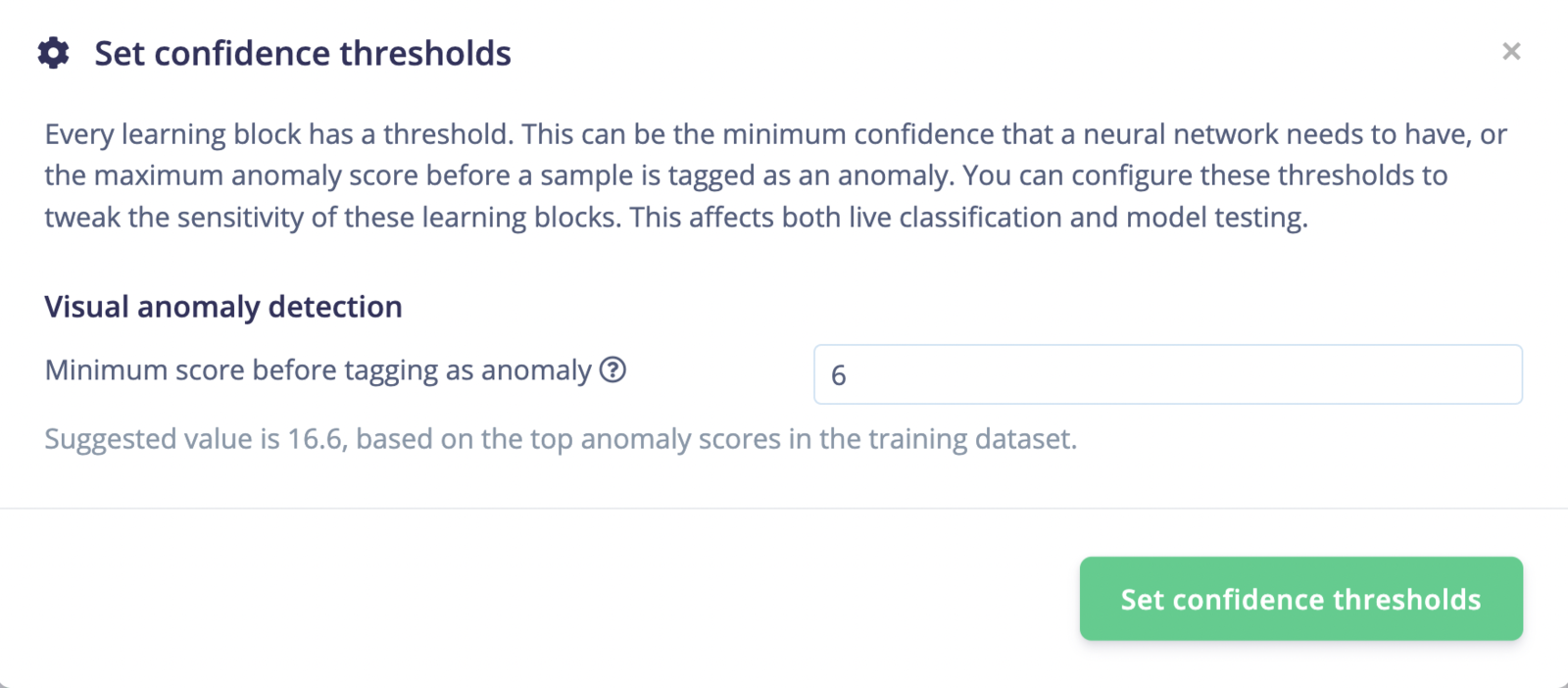
In this project, we have set the confidence threshold to 6. This gives results closer to our expectations:

Model testing view and sample selected after confidence thresholds modified.

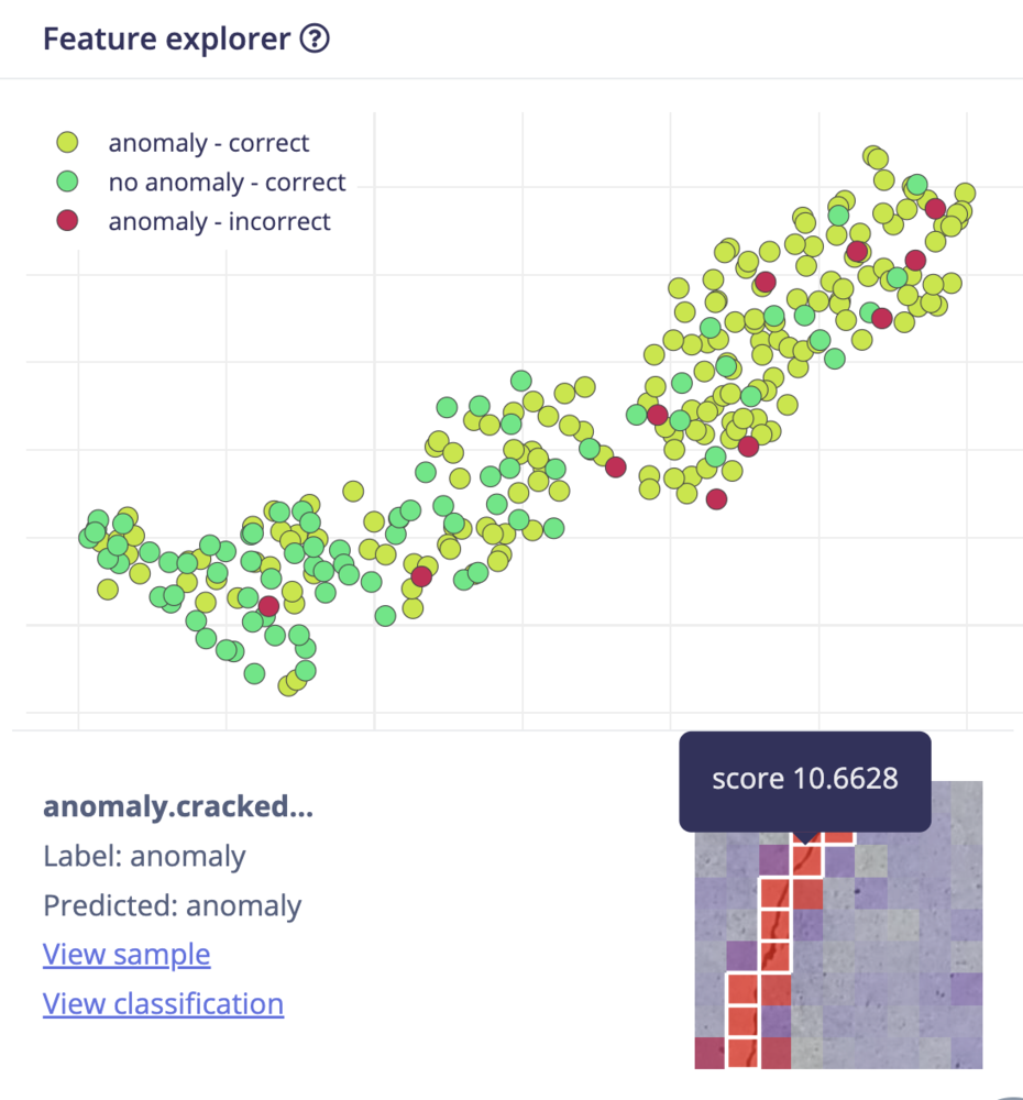
• Cells with white borders are the ones that passed as anomalous, given the confidence threshold of the learning block.

• All cells are assigned a cell background color based on the anomaly score, going from blue to red, with an increasing opaqueness.

• Hover over the cells to see the scores.

• The grid size is calculated as (inputWidth / 8) / 2 - 1 for GMM and as inputWidth / 8 for Patchcore.

Keep in mind that every project is different, and will thus use different suggested confidence thresholds depending on the input training data, please make sure to also validate your results in real conditions. The suggested threshold is np.max(scores) where scores are the scores of the training dataset.

Additional resources

Interesting readings:

• Python Data Science Handbook - Gaussian Mixtures
• scikit-learn.org - Gaussian Mixture models
• PatchCore - Towards Total Recall in Industrial Anomaly Detection

Public projects:

• Visual GMM cracks
• Thermostatic valve (FOMO-AD 96x96) - dataset collected by Edge Impulse