Only available for Audio data projectsPerformance calibration is only available for projects that contain audio data. It’s designed for use with projects that are detecting specific events (such as spoken keywords), as opposed to classifying ambient conditions.
What does Performance Calibration do?
Performance Calibration is a tool for testing and configuring embedded machine learning pipelines for event detection. It provides insight into how your pipeline will perform on streaming data, which is what your application will encounter in the real world. It works within Studio, and does not require you to deploy to a physical device. After testing is complete, you can use Performance Calibration to configure a post-processing algorithm that will interpret the output of your ML pipeline, transforming it into a stream of actionable events. The results of testing are used to help guide selection of the optimal post-processing algorithm for your use case. For example, a developer working on a keyword spotting application could use Performance Calibration to understand how well their ML pipeline detects keywords in a sample of real world audio, and to select the post-processing algorithm that provides the best quality output.Understanding Post-processing:
Post-processing is the technique used to refine the raw outputs from your impulse, transforming them into actionable insights. Here’s how it’s done: Averaging Scores Over a Window: Before any decisions are made, the model’s output scores are averaged over a specified duration to smooth out any abrupt fluctuations. Applying a Threshold: Only the top score, after averaging, is considered. If this score surpasses a predetermined threshold, it indicates the presence of a detected event. Suppression Period: After a positive event detection, there’s a period where any subsequent detections are temporarily ignored. This avoids rapid repeated detections of the same event and reduces false positives.Post-processing algorithm
The post-processing algorithm has a configurable set of parameters that determine the overall performance of the pipeline. These parameters can be adjusted to control the trade-off between false acceptance rate (how often an event is mistakenly detected) and false rejection rate (how often an event is mistakenly ignored). This allows you to determine how sensitive your impulse is to inputs. Your impulse can be tailored using a specific post-processing configuration. This configuration can be adjusted to minimize either false activations (False Alarm Rate - FAR) or false rejections (False Rejection Rate - FRR). The UI provides a chart showcasing a range of recommended configurations. Once you find a configuration that meets your criteria, you can save it, ensuring it’s applied whenever the impulse is deployed.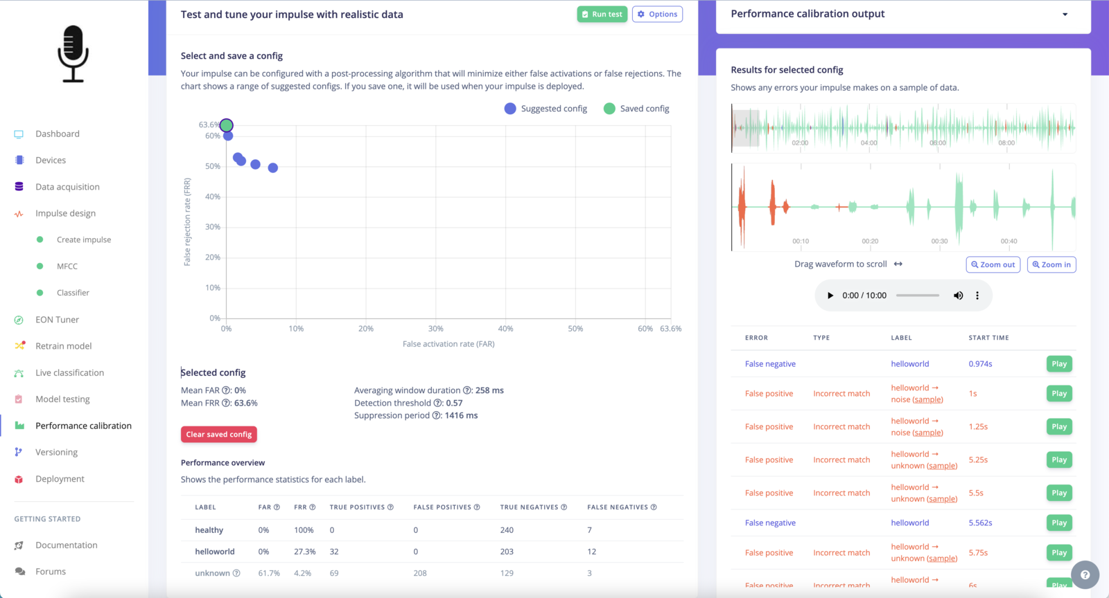
Mean FAR (False Alarm Rate):
The percentage of times the system wrongly identified an event.Mean FRR (False Rejection Rate):
The percentage of times the system failed to identify an event.Averaging window duration:
The duration over which the model’s output scores are averaged to smooth out any abrupt fluctuations.Detection threshold:
The minimum score required to indicate the presence of a detected event.Suppression period:
The duration after a positive event detection where any subsequent detections are temporarily ignored. This avoids rapid repeated detections of the same event and reduces false positives.Why is it useful?
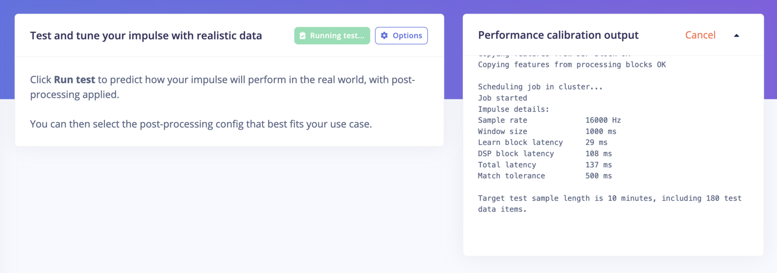
Performance Calibration gives you an accurate prediction of how your ML pipeline will perform when it is deployed in the real world. Analyzing real world performance before deployment in the field allows you to iterate on your pipeline much more quickly, helping you identify and solve common performance issues much earlier in the process. Interpreting the output of an ML pipeline on streaming data requires a post-processing algorithm, which edge ML developers have traditionally had to write and tune by hand, balancing the trade-off between false positives and false negatives to fit their particular use case. By quantifying and automating this process, Performance Calibration gives developers precise control over the trade-offs they select for their application.How does it work?
Performance can be measured using either recordings of real-world data, or with realistic synthetic recordings generated using samples from your test dataset. This allows you to easily test your model’s performance under various scenarios, such as varying levels of background noise, or with different environmental sounds that might occur in your deployment environment. When Performance Calibration runs, your ML pipeline is run across the input data with the same latency as is predicted for the target selected on the Dashboard page of your project. This results in a set of raw predictions which must be filtered by a post-processing algorithm to produce a signal every time a particular event class is detected. The post-processing algorithm has configurable parameters that determine the overall performance of the pipeline. These parameters can be adjusted to control the trade-off between false acceptance rate (how often an event is mistakenly detected) and false rejection rate (how often an event is mistakenly ignored). This allows you to determine how sensitive your application is to inputs.False positives and false negativesNo ML model is perfect, so developers using ML for event detection always need to pick a trade-off between false positives and false negatives. The appropriate trade-off depends on the application. For example, if you’re attempting to detect a dangerous situation in an industrial facility, it may be important to minimize false negatives. On the other hand, if you’re concerned about annoying users with unintentional activations of a smart home device, you may wish to minimize false positives.
Test configuration
First, make sure you have an audio project in your Edge Impulse account. No projects yet? Follow one of our tutorials to get started: Or, clone the “Bird sound classifier” project that is used in this documentation to your Edge Impulse account: https://studio.edgeimpulse.com/public/16060/latest Once you’ve trained your impulse, select the Performance calibration tab and set your testing configuration settings: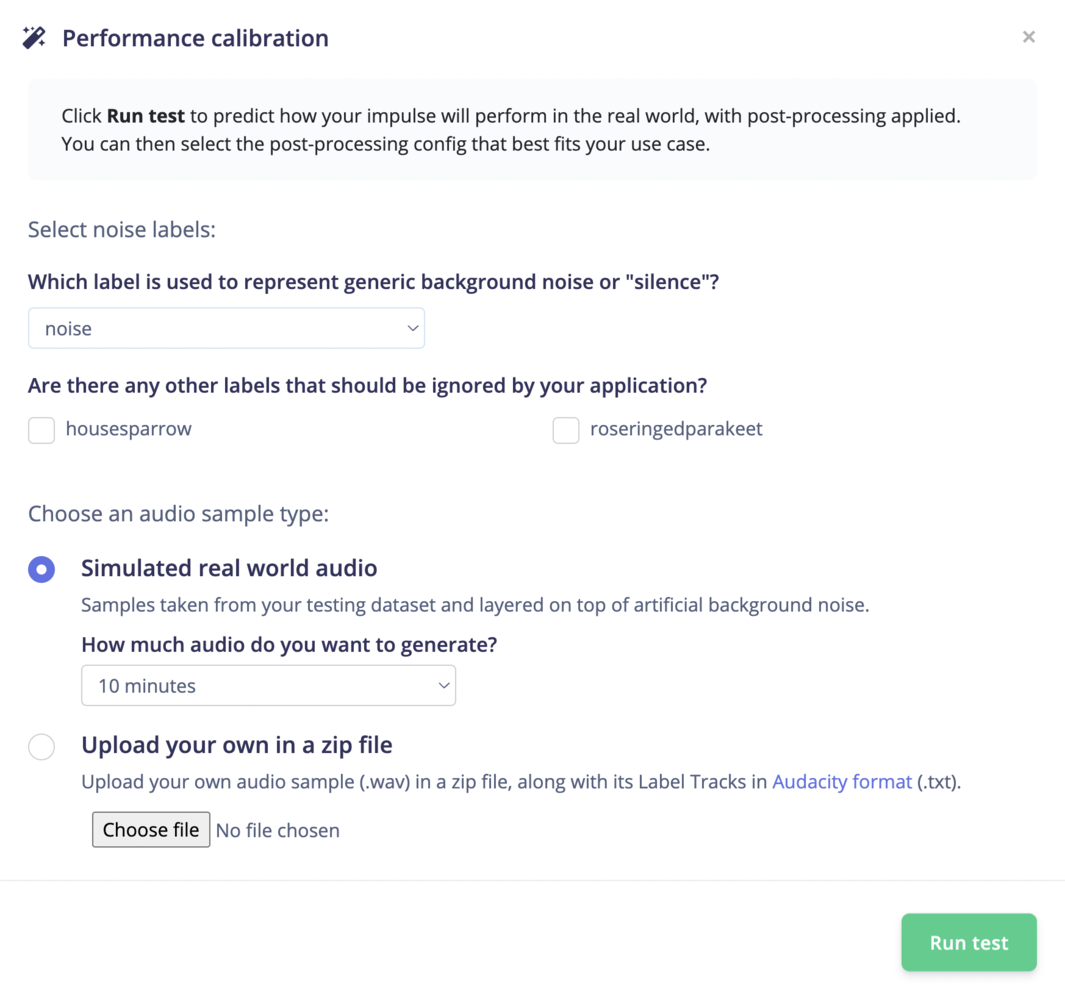
- Select noise labels. Which label is used to represent generic background noise or “silence”?
- Select any other labels that should be ignored by your application, i.e. other classes that are equivalent to background noise or “silence”.
- Choose an audio sample type: simulated real world audio or upload your own in a zip file.
- Then, click Run test.
Simulated real world audio
Simulated real world audio is a synthetically generated audio stream consisting of samples taken from your testing dataset and layered on top of artificial background noise. For free Edge Impulse projects, you can choose to generate either 10 minutes or 30 minutes of simulated real world audio.Upload your own in a zip file
Already have a long, real-world recording of background noise which includes your target model’s classes? Upload your own audio sample (.wav) in a zip file, along with its Label Tracks in Audacity format (.txt).Select and save a config
Your impulse can be configured with a post-processing algorithm that will minimize either false activations or false rejections. The chart shows a range of suggested configs. If you save one, it will be used when your impulse is deployed.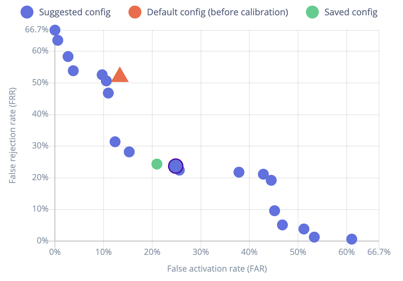
Selected config
Selecting from the various “Suggested config” icons on the FRR/FAR chart will update the Selected config information. Click on Save selected config to use the selected FAR and FRR trade off when your impulse is deployed. This config information is also accessible in the deployed Edge Impulse library.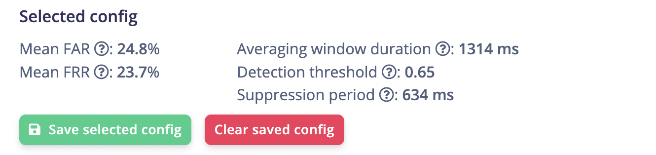
- Mean FAR: The mean False Acceptance Rate. Measures how often labels are mistakenly detected. Does not include statistics for noise labels.
- Mean FRR: The mean False Rejection Rate. Measures how often events are mistakenly missed. Does not include statistics for noise labels.
- Averaging window duration (ms): The raw inference results are averaged across this length of time.
- Detection threshold (ms): A class is considered a positive match when it exceeds this threshold.
- Suppression period (ms): Matches are ignored for this length of time following a positive result.
Performance overview
Shows the performance statistics for each label.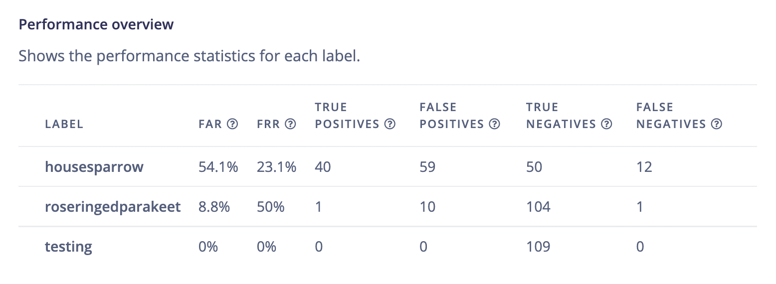
- FAR: False Acceptance Rate. Measures how often a label is mistakenly detected.
- FRR: False Rejection Rate. Measures how often a label is mistakenly missed.
- True Positives: The number of times each label was correctly triggered.
- False Positives: The number of times each label was incorrectly triggered.
- True Negatives: The number of times each label was correctly not triggered.
- False Negatives: The number of times each label was incorrectly not triggered.
False acceptance rate and false rejection rateFAR is also sometimes known as the False Positive Rate, and FRR as the False Negative Rate. These industry-standard metrics are calculated as follows:
Results for selected config
Shows any errors your impulse makes on a sample of data, with a table of results.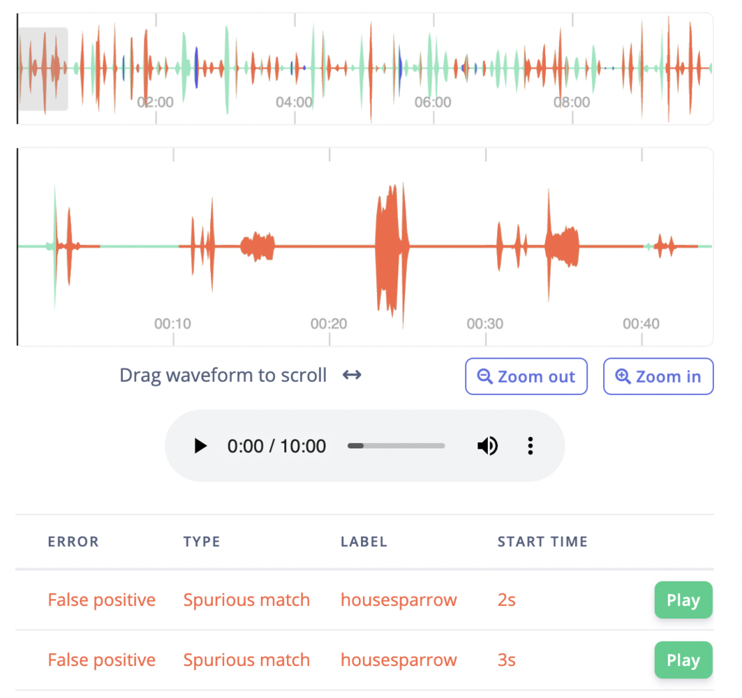
- Error: False positives are displayed in red while false negatives are displayed in blue.
- Type: Spurious match, incorrect match, duplicate match, or blank.
- Label: The data label the model predicted in the audio stream.
- Start time: The timestamp starting location of the selected error in the audio data stream.
- Play button: Preview the audio stream at the error’s start time.
Types of false positives
What we refer to as “Ground Truth” in this context is the sound/label association that the synthetically generated audio contains at a given time.- Incorrect match: A detection matches the wrong ground truth
- Spurious match: This match detection has not been associated with any ground truth.
- Duplicate match: The same ground truth was detected more than once. The first correct detection is considered a true positive but subsequent detections are considered false positives.