Spectral features parameters overview
Spectral analysis parameters
Compatible with the DSP Autotuner
Picking the right parameters for DSP algorithms can be difficult. It often requires a lot of experience and experimenting. The autotuning function makes this process easier by looking at the entire dataset and recommending a set of parameters that is tuned for your dataset.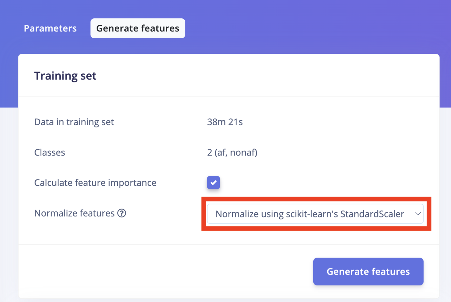
Normalize features
Filter
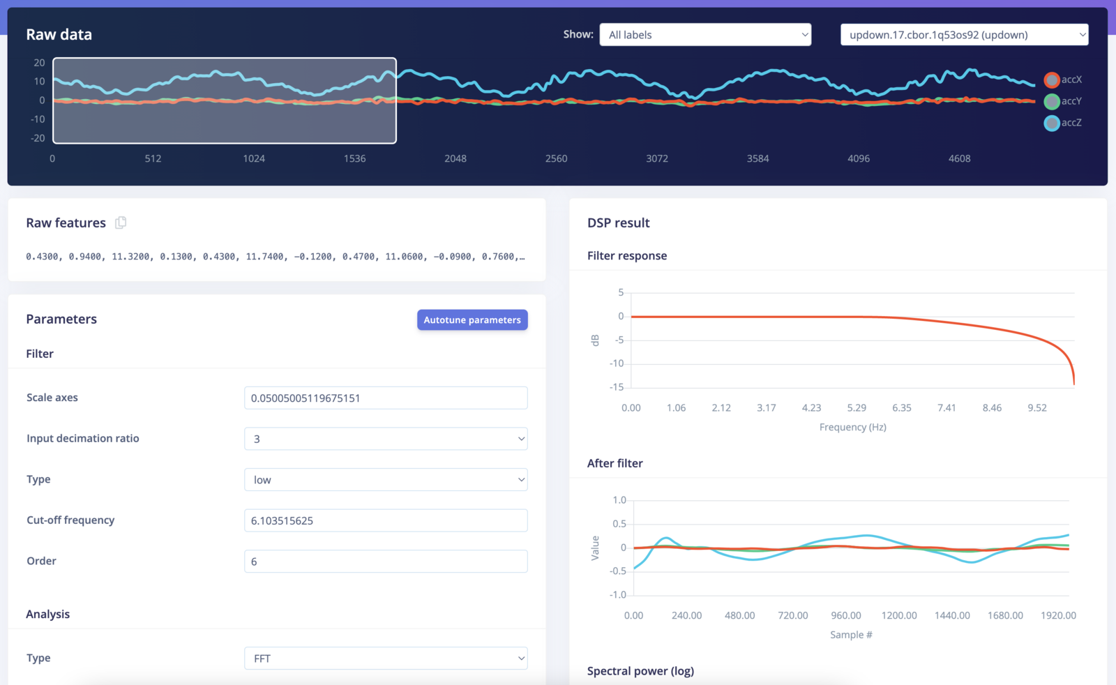
Prior to calculating the Fast Fourier Transform (FFT), the time-series data inside the window of your sample can be filtered, which often helps to smooth out the signal or drop unwanted artifacts. In the image above, a “window” is shown inside the white box; only the readings inside that box will be used for filtering and calculating the FFT. Edge Impulse will slide the window over your sample, as given by the time series input block parameters during Impulse creation in order to generate several training/test samples from your longer time series sample.- Scale axes - Multiply all raw input values by this number.
- Input decimation ratio - Decimating (downsampling) the signal reduces the number of features and improves frequency resolution in relevant bands without increasing resource usage.
- Type - The type of filter to apply to the raw data (low-pass, high-pass, or none).
- Cut-off frequency - Cut-off frequency of the filter in hertz. Also, this will remove unwanted frequency bins from the generated features.
- Order - Order of the Butterworth filter. Must be an even number. A higher order has a sharper cutoff at the expense of latency. You can also set to zero, in which case, the signal won’t be filtered, but unwanted frequency bins will still be removed from the output.
Removing frequency bins beyond the cut off reduces model size, which saves resources, and also leads to models that train well with less data
Analysis - Spectral power
Analysis type - There are two types of analysis you can choose from.
- FFT base analysis is best at analyzing repetitive patterns in a signal,
- Wavelet works better for complex signals that have transients or irregular waveform.
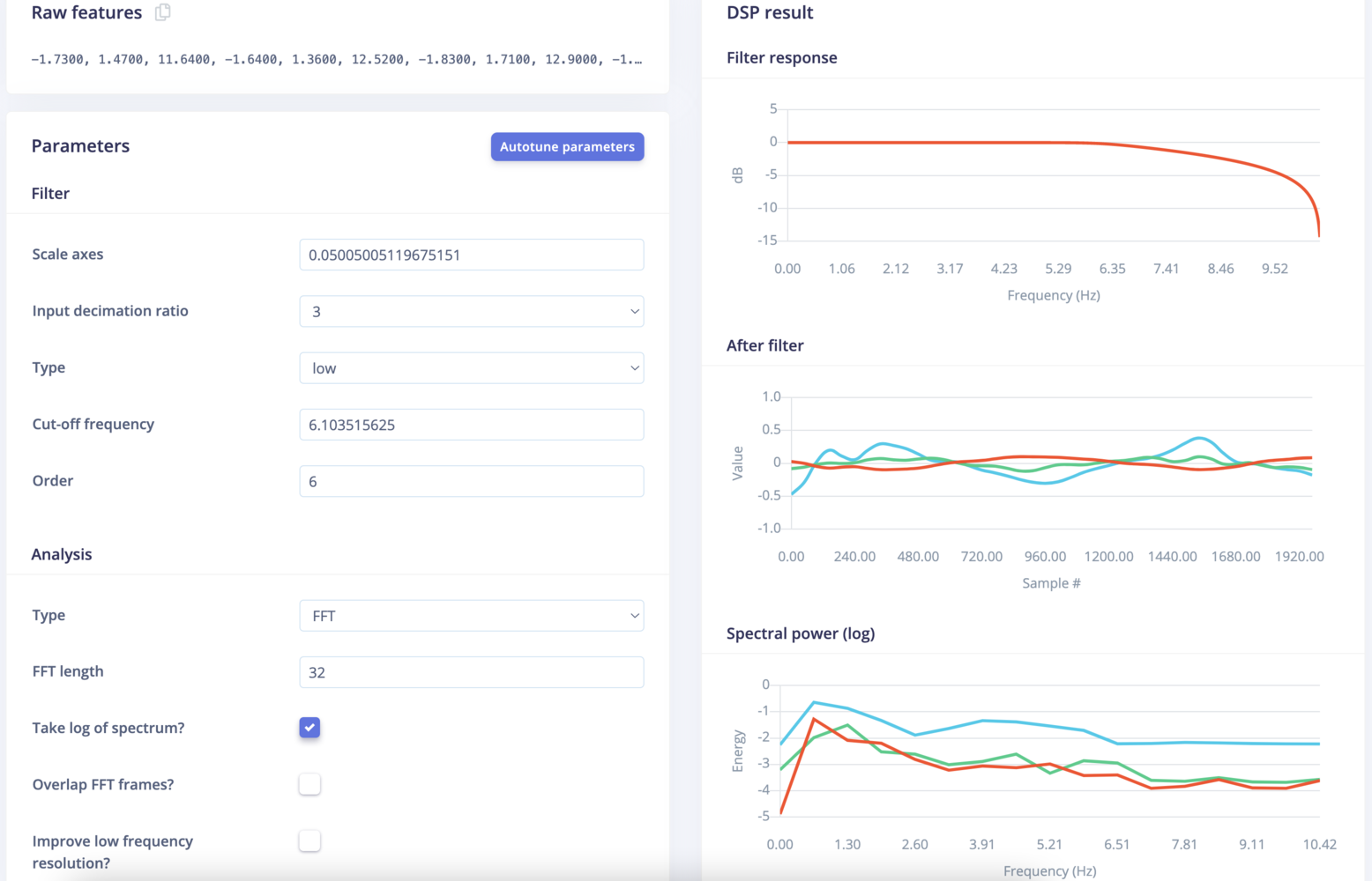
FFT
- FFT length - The FFT size. This determines the number of FFT bins as well as the resolution of frequency peaks that you can separate. A lower number means more signals will average together in the same FFT bin, but also reduces the number of features and model size. A higher number will separate more signals into separate bins, but generates a larger model.
- Take log of spectrum? - When selected, log (base 10) will be applied to each FFT bin. This gives more range to (ie, captures more information about) low intensity signals at the expense of range for higher intensity signals. It is enabled by default and is generally a good choice, but it ultimately depends on the kind if signal sampled.
- Overlap FFT frames? - Successive frames (sub-windows) overlap by 1/2 within the larger window (given by the white box in the image) if this is checked. If unchecked, frames will not overlap. This “sliding frame” method can prevent transient events from being missed if they happen to appear on a frame boundary. Enabled by default. Disabling improves latency. No impact on model size or RAM usage.
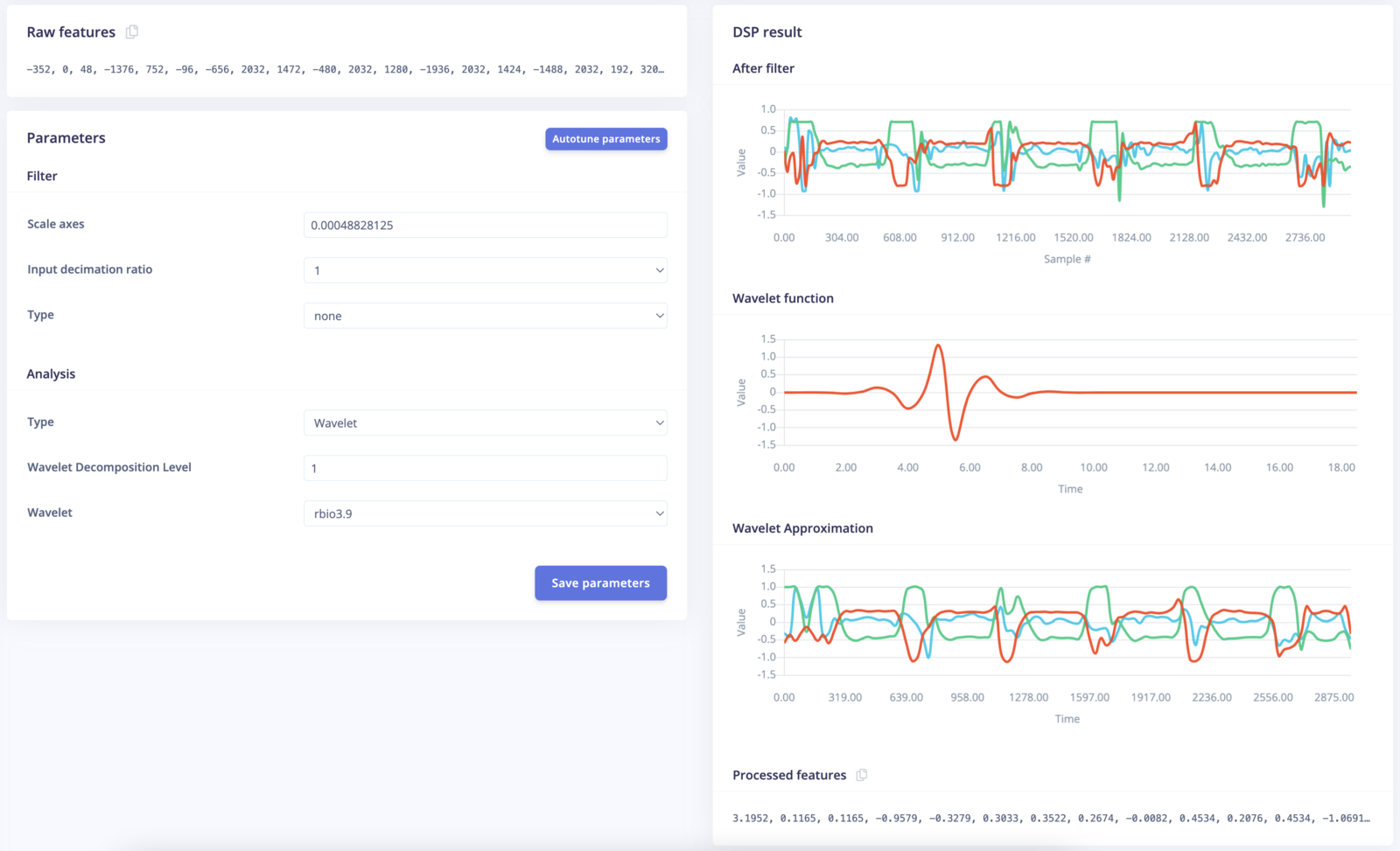
Wavelet
- Wavelet decomposition level The level at which you wish to decompose the signal. Higher level reveals more information about the signal at a cost of more computing requirement and may introduce noise due to numerical precision limitations.
- Wavelet The wavelet kernel. There are many types of wavelet to choose from, the best choice is often the one that mimics the pattern of interests in the signal.
Graphs
- Filter response - If filtering is enabled, and order is non-zero, then the frequency response of the filter is shown. This shows how much attenuation there will be across the frequency spectrum.
- After filter - Shows the current window after filtering is applied (in the time domain).
- Spectral power - Shows power vs. frequency as computed by the chosen FFT size. Power is either linear or log based on settings. This is shown if the selected analysis type is FFT.
- Wavelet function - Shows the wavelet kernel function. This is shown if the selected analysis type is Wavelet.
- Wavelet approximation - Shows the approximation of the signal at the highest decomposition level. This is shown if the selected analysis type is Wavelet.
Output features of the spectral analysis block
Using FFTs: The spectral analysis block generates 2 types of features per axis/channel:- Statistical features
- RMS
- Skewness
- Kurtosis
- Spectral features
- Maximum value from FFT frames for each bin that was not filtered out
For example, let’s consider an input signal sampled at 62.5 Hz with 3 axis and the following parameters:
- Low-pass filter
- Filter cutoff set to 3 Hz
- 3 values for statistics (RMS, Skewness, Kurtosis)
- 1 value for the FFT bin capturing 1.95 to 5.86 Hz
- Entropy
- Zero cross
- Mean cross
- 5 percentile
- 25 percentile
- 75 percentile
- 95 percentile
- Median
- Mean
- Stdev
- Variance
- RMS
- Skewness
- Kurtosis
For example, for a 4-level decomposition, with 14 features per component, it will generate 70 features in total.