Features importance (optional)
In most of our DSP blocks, you have the option to calculate the feature importance. Edge Impulse Studio will then output a Feature Importance list that will help you determine which axes generated from your DSP block are most significant to analyze when you want to do anomaly detection. See Processing blocks > Feature importanceSetting up the Anomaly Detection (GMM) learning block
The GMM anomaly detection learning block has two adjustable parameters: the Number of components and The axes.Number of components
The number of (gaussian) components can be interpreted as the number of clusters in Gaussian Mixture Models.How to choose the number of components?When increasing the number of (Gaussian) components, the model will fit the original distribution more closely. If the value is too high, there is a risk of overfitting.If you have prior knowledge about the problem or the data, it can provide valuable insights into the appropriate number of components. For example, if you know that there are three distinct groups in your data, you may start by trying a GMM with three components. Visualizing the data can also provide hints about the number of clusters. If you can distinguish several visible clusters from your training dataset, try to set the number of components as the number of visible clusters
Axes
The different axes correspond to the generated features from the pre-processing block. The chosen axes will use the features as the input data for the training.Click on the Select suggested axes button to harness the results of the feature importance output.
Train
Click on Start training to trigger the learning process. Once trained you will obtain a view that looks like the following: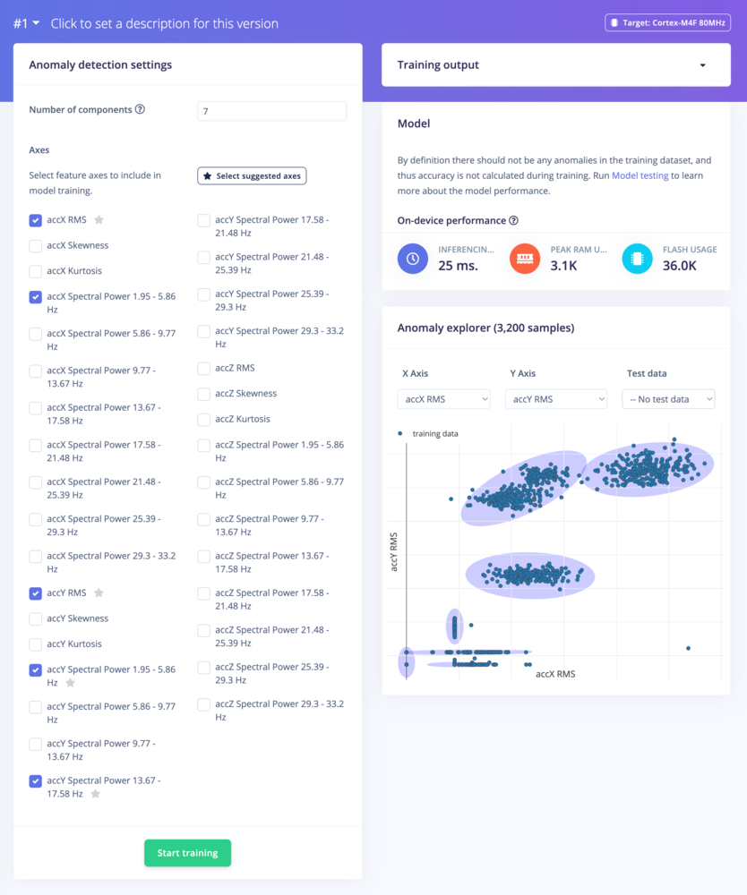
GMM learning block trained
Testing single sample
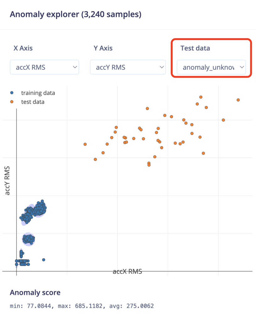
Testing the Anomaly Detection (GMM) learning block
Navigate to the Model testing page and click on Classify all: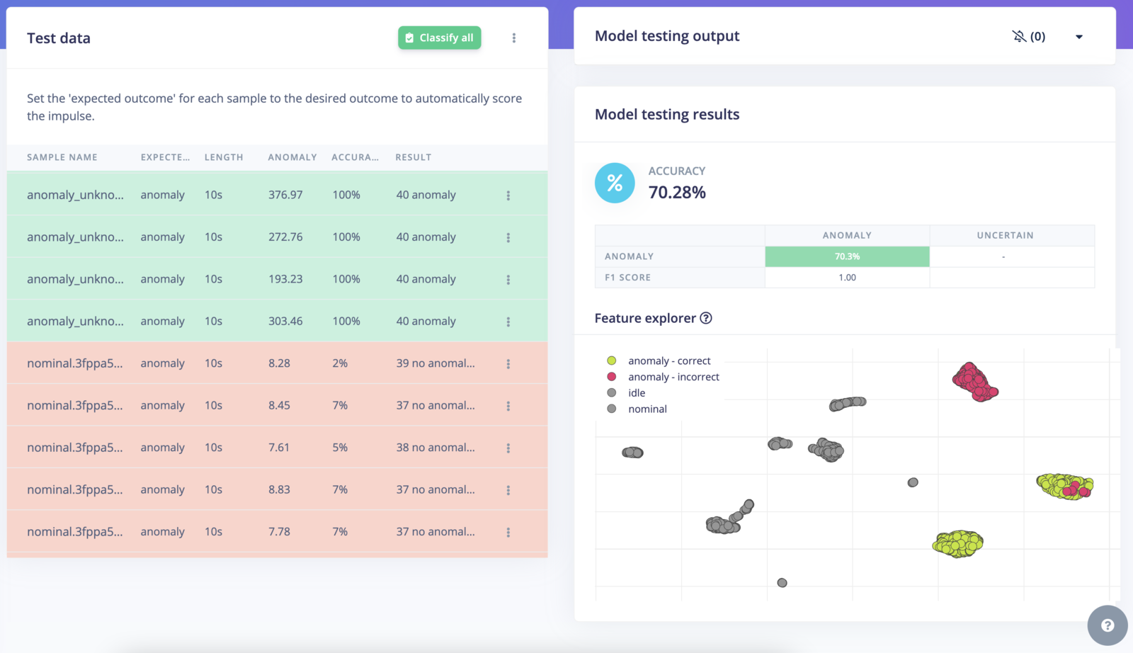
Model testing view
Confidence threshold
In the example above, you will see that some samples are considered asno anomaly while the expected output is an anomaly. If you take a closer look at the anomaly score for non anomaly samples, the range values are below 1.00:
Model testing view
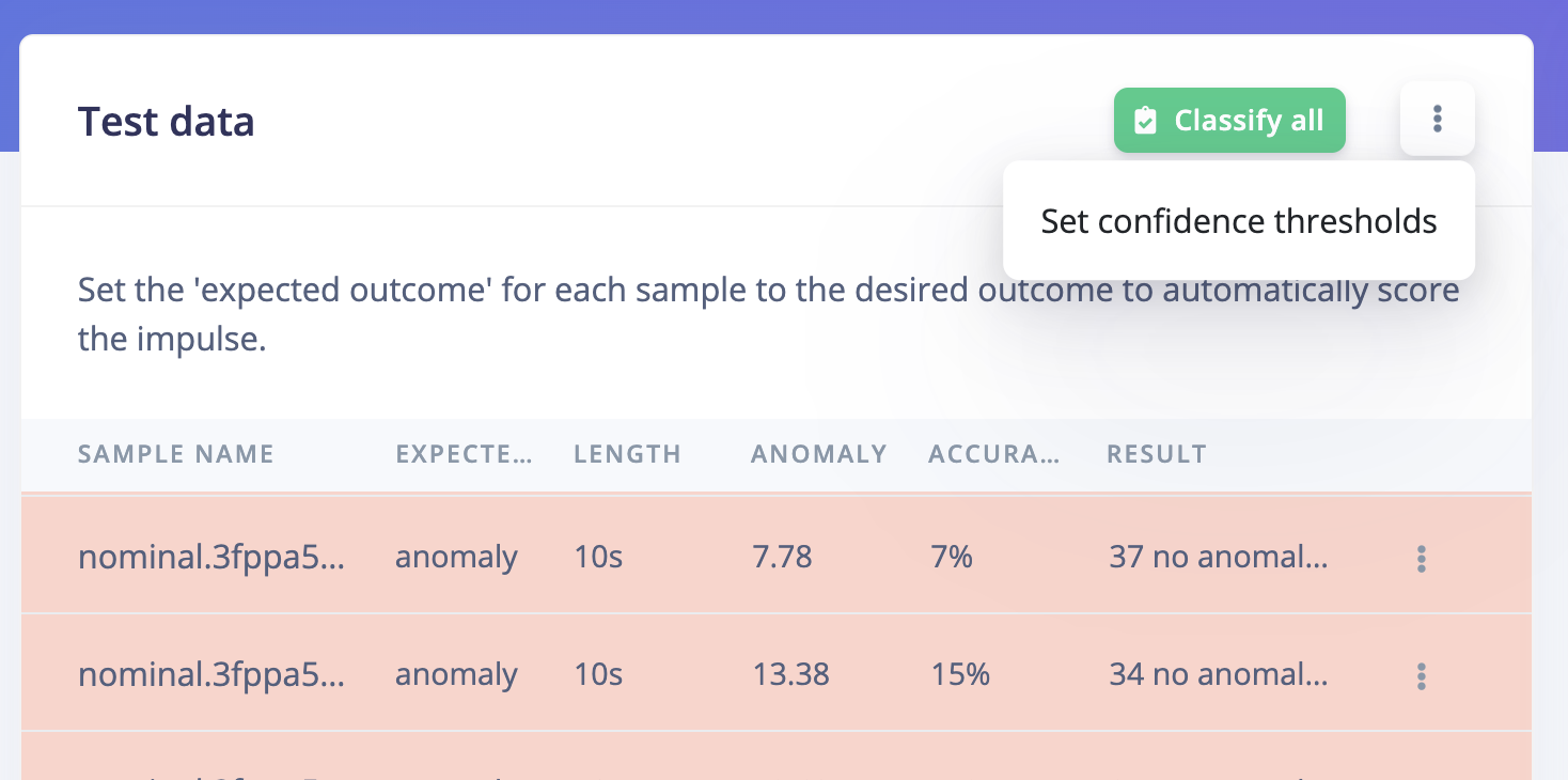
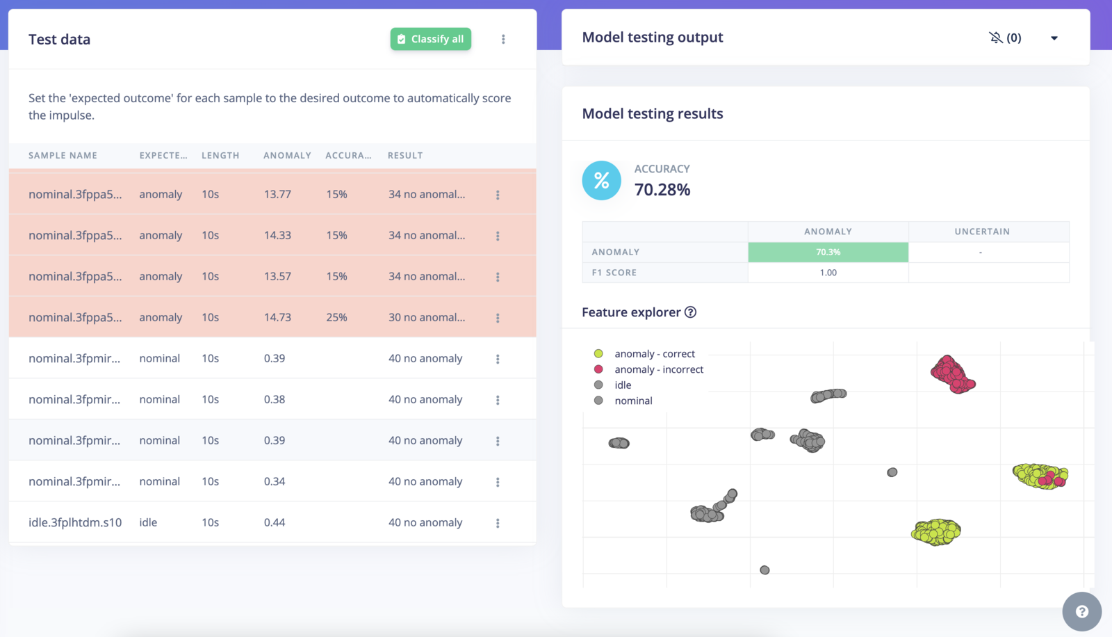
Setting confidence threshold
1.00. This gives results closer to our expectations:
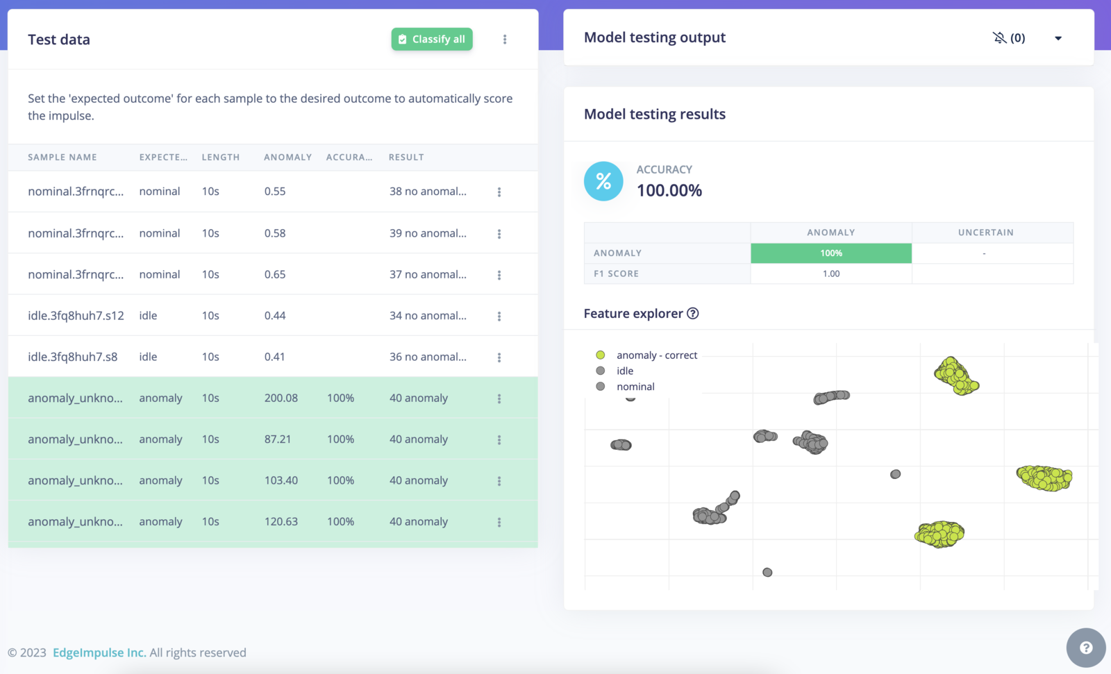
Model testing view
How does it work?
- During training, X number of Gaussian probability distributions are learned from the data where X is the number of components (or clusters) defined in the learning block page. Samples are assigned to one of the distributions based on the probability that it belongs to each. We use Sklearn under the hood and the anomaly score corresponds to the
log-likelihood. - For the inference, we calculate the probability (which can be interpreted as a distance on a graph) for a new data point belonging to one of the populations in the training data. If the data point belongs to a cluster, the anomaly score will be low.
Additional resources
Interesting readings:- Python Data Science Handbook - Gaussian Mixtures
- scikit-learn.org - Gaussian Mixture models