

Introduction
Industrial machines don’t become obsolete just because technology moves forward. Factory floors are already full of PLCs, controllers, and sensors that have been running reliably for years, quietly generating production data that never leaves the machine. That data is valuable, but it’s often locked behind proprietary protocols and isolated industrial networks, out of reach of the cloud, IoT, and AI tools that could actually put it to use. The Edge Link project have been created to change that.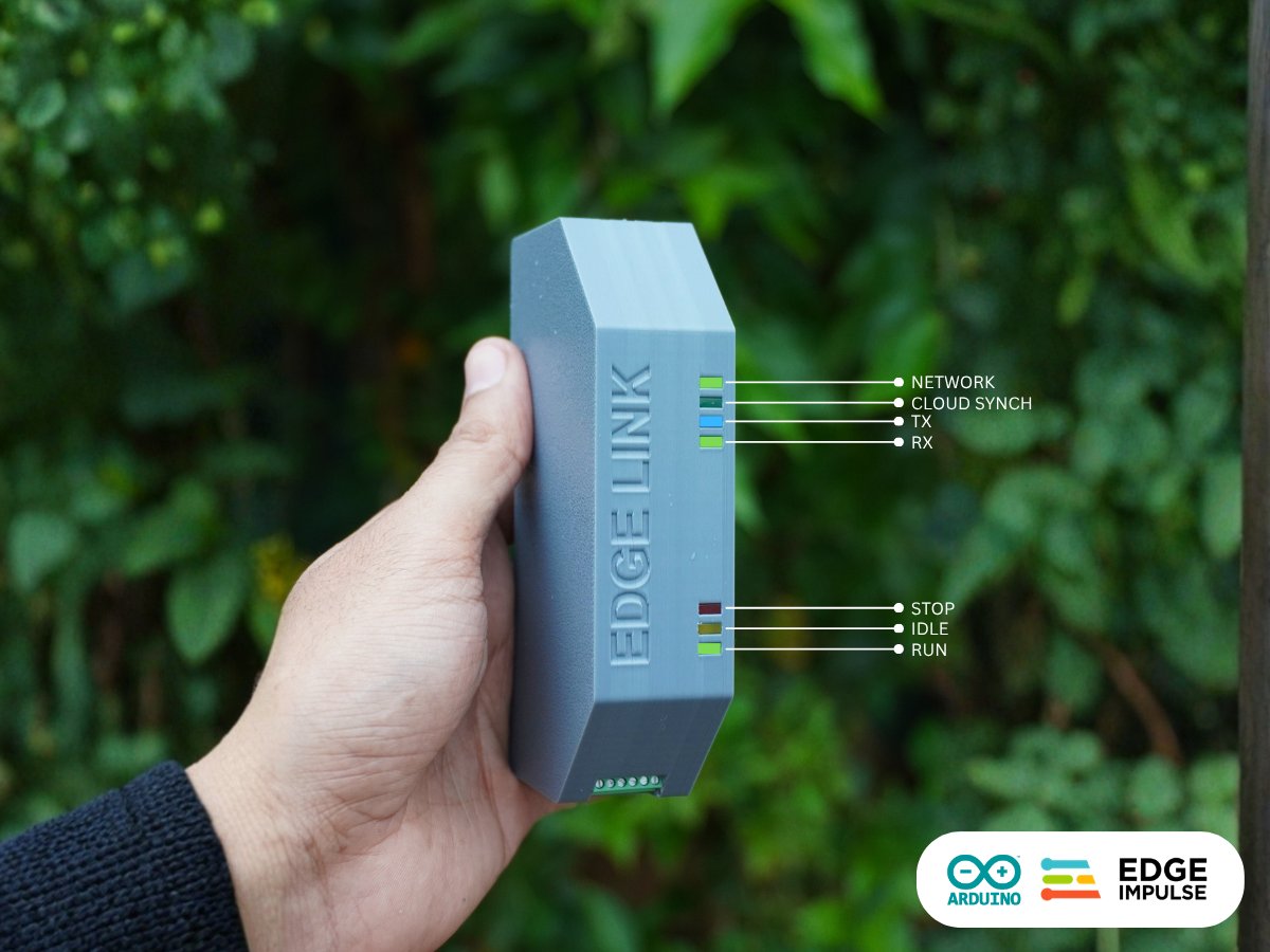
Edge Impulse ML Models
Now let’s come to the Edge Impulse ML models running on the Arduino UNO Q. The Edge Link application package already contains six pre-trained Edge Impulse models, one for each production-line station:pm_st1.eim: Station 1pm_st2.eim: Station 2pm_st3.eim: Station 3pm_st4.eim: Station 4pm_st5.eim: Station 5pm_e1.eim: Overall/production-line model
How the Predictive Maintenance Models Work?
Each model is designed for a specific part of the production line and expects a particular set of input features. For example, Station 1 – PCB Assembly uses thepm_st1.eim model.
The model monitors parameters such as:
Model Outputs
The Station 1 model can classify the machine condition into states such as:normal, warning, and fault conditions. These allow the simulator to generate different machine-health conditions and provide the corresponding feature values to the model.
Real-Time Inference on the Arduino UNO Q
The important part is that the ML inference is performed locally on the Arduino UNO Q. The PLC Simulator continuously generates the machine data and sends the formatted data to the Edge Link. The Edge Link identifies the station and extracts the required features for that station’s model. For example:PLC Simulator
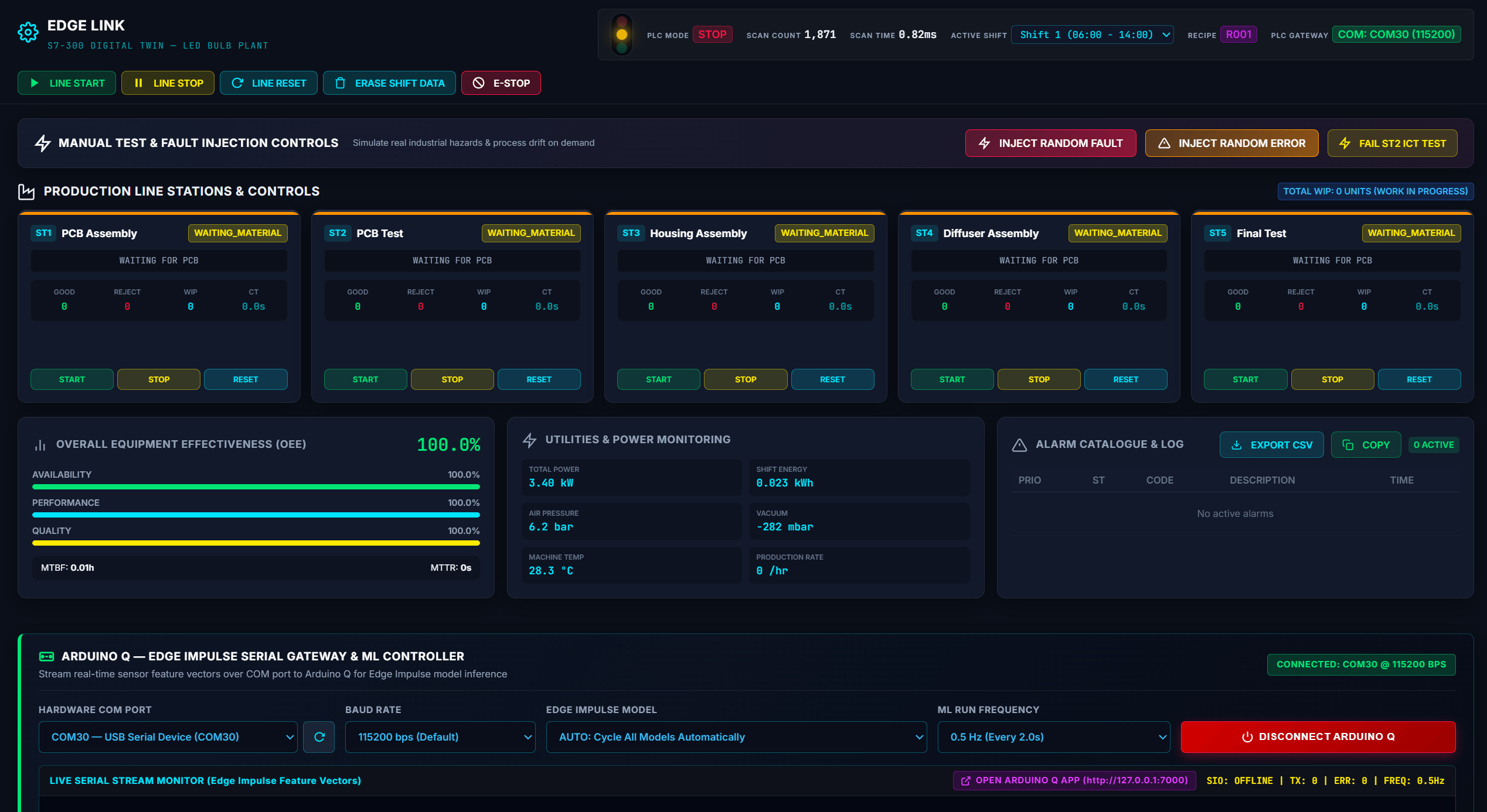
→ Station 1 sensor data → Edge Link → pm_st1.eim → Arduino UNO Q → Predictive-maintenance inference → Machine-health result
This happens in milliseconds, allowing the system to continuously monitor the health of the production equipment without sending every inference request to the cloud.
So instead of having a single ML model monitoring the entire factory, we have station-specific predictive-maintenance models running as part of the Edge AI pipeline.
This is where the MCU + MPU architecture of the Arduino UNO Q becomes particularly useful. We are not simply collecting data and forwarding it to the cloud. We are continuously processing machine data at the edge and performing predictive maintenance inference locally.
The cloud can still be used for historical data, visualization, analytics, and long-term monitoring, while the UNO Q provides the low-latency Edge AI layer.
Training Custom AI Models in Edge Impulse
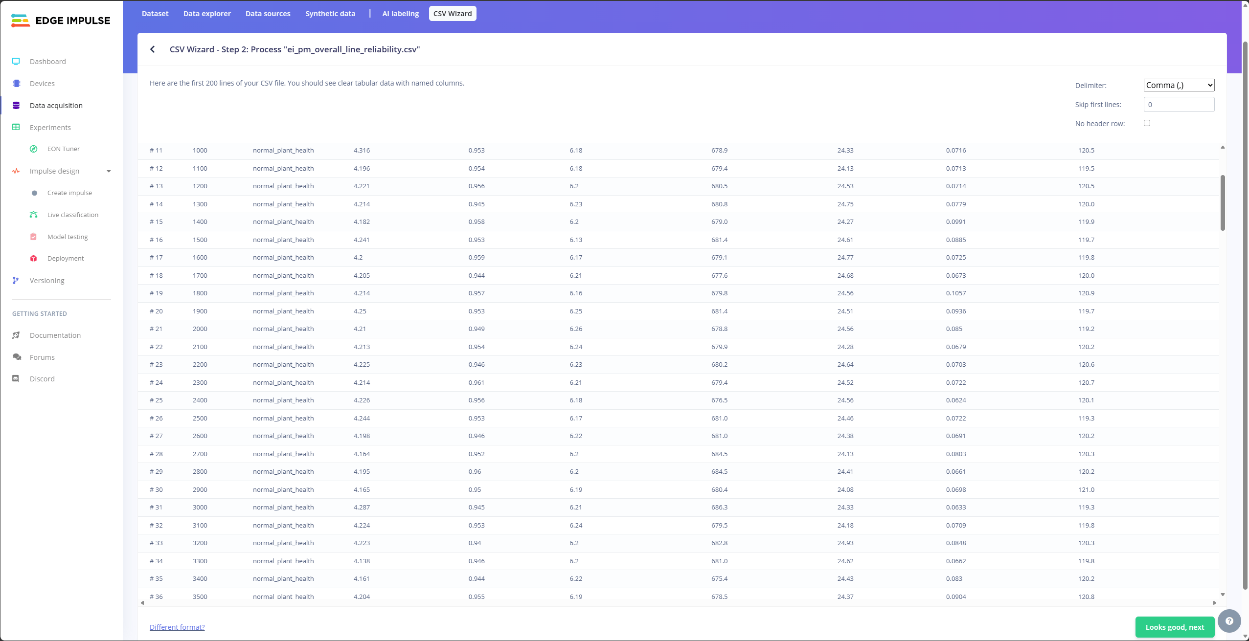
Now that we have seen how the pre-trained Edge Impulse models work, let’s look at how we can build our own predictive-maintenance models using Edge Impulse. The first requirement for training an ML model is a large and representative dataset. Since we don’t have access to a real production line, we can use our PLC Simulator to generate realistic simulated machine data. The PLC Simulator includes a dedicated Edge Impulse Data Generator directly inside the SCADA web application. One hour of simulated production generates 36,000 samples at 10 Hz in less than 0.2 seconds, giving us a very fast way to generate large datasets without having to wait for a real production line to operate for hours. The generated dataset is imported into Edge Impulse via theCSV Wizard (Data Acquisition > CSV Wizard > Upload CSV), configured as time-series data with a timestamp column in elapsed milliseconds and the machine-health condition selected from the label column, with a sample length of 2000 ms.
Generate the Dataset from the PLC Simulator
The PLC Simulator includes a dedicated Edge Impulse Data Generator directly inside the SCADA web application. Open the PLC Simulator SCADA interface and selectEdge Impulse Data Generator
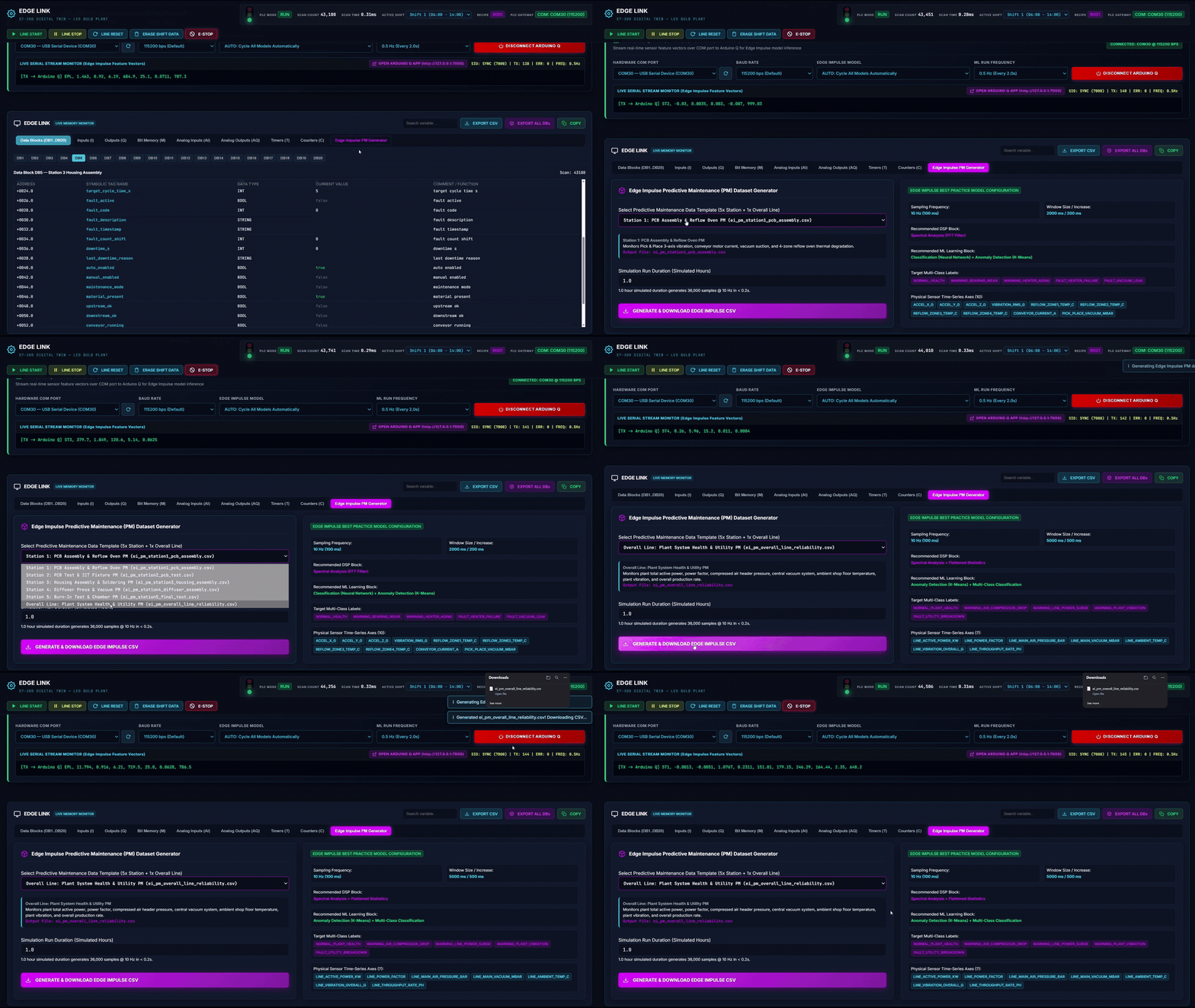
- Select the station/model dataset you want to generate.
- Enter the required simulation run duration.
- Click Generate.
Create an Edge Impulse Project
Now let’s import this dataset into Edge Impulse. Go to the Edge Impulse Studio, sign in with your account, and create a new project.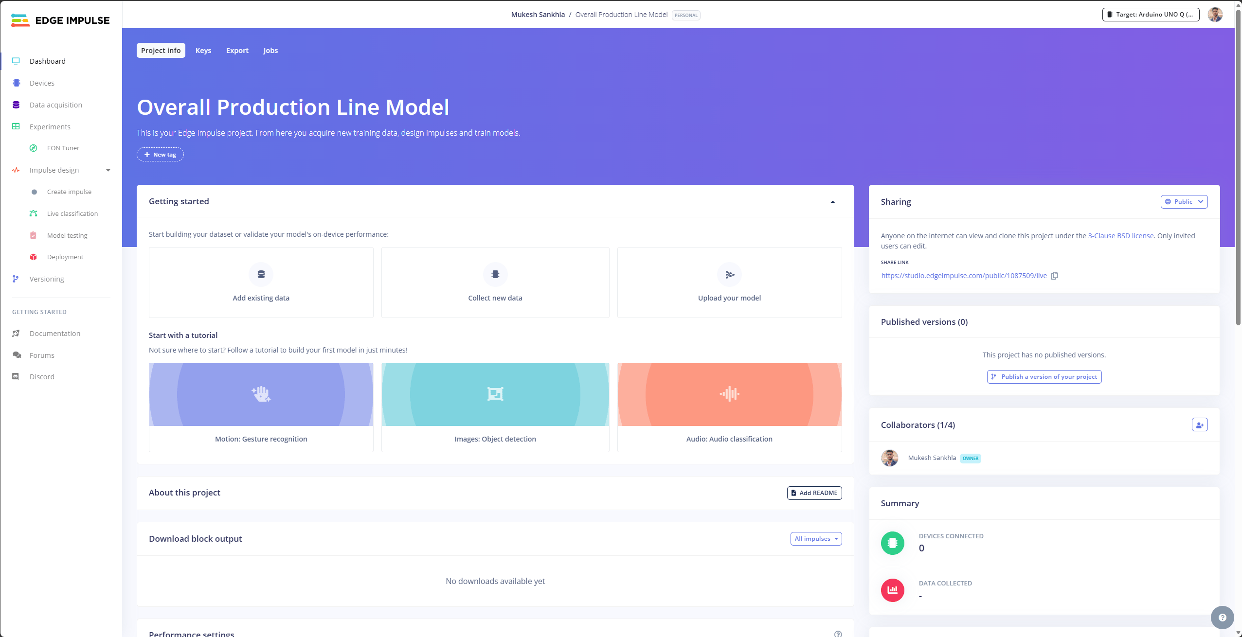
Import the CSV Using CSV Wizard
Inside the Edge Impulse project, go to Data Acquisition.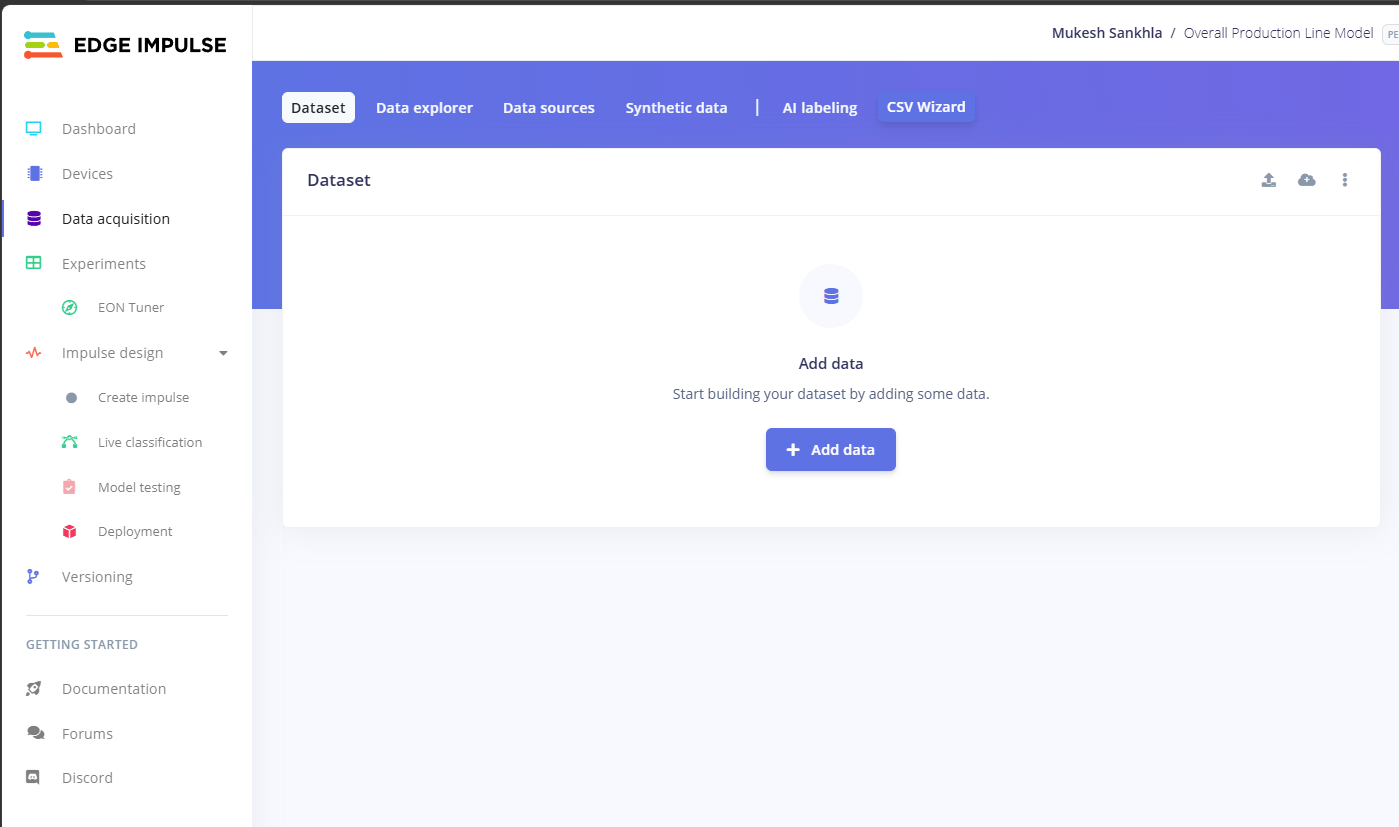
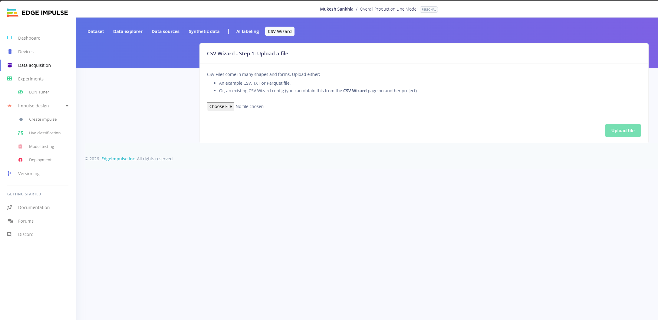
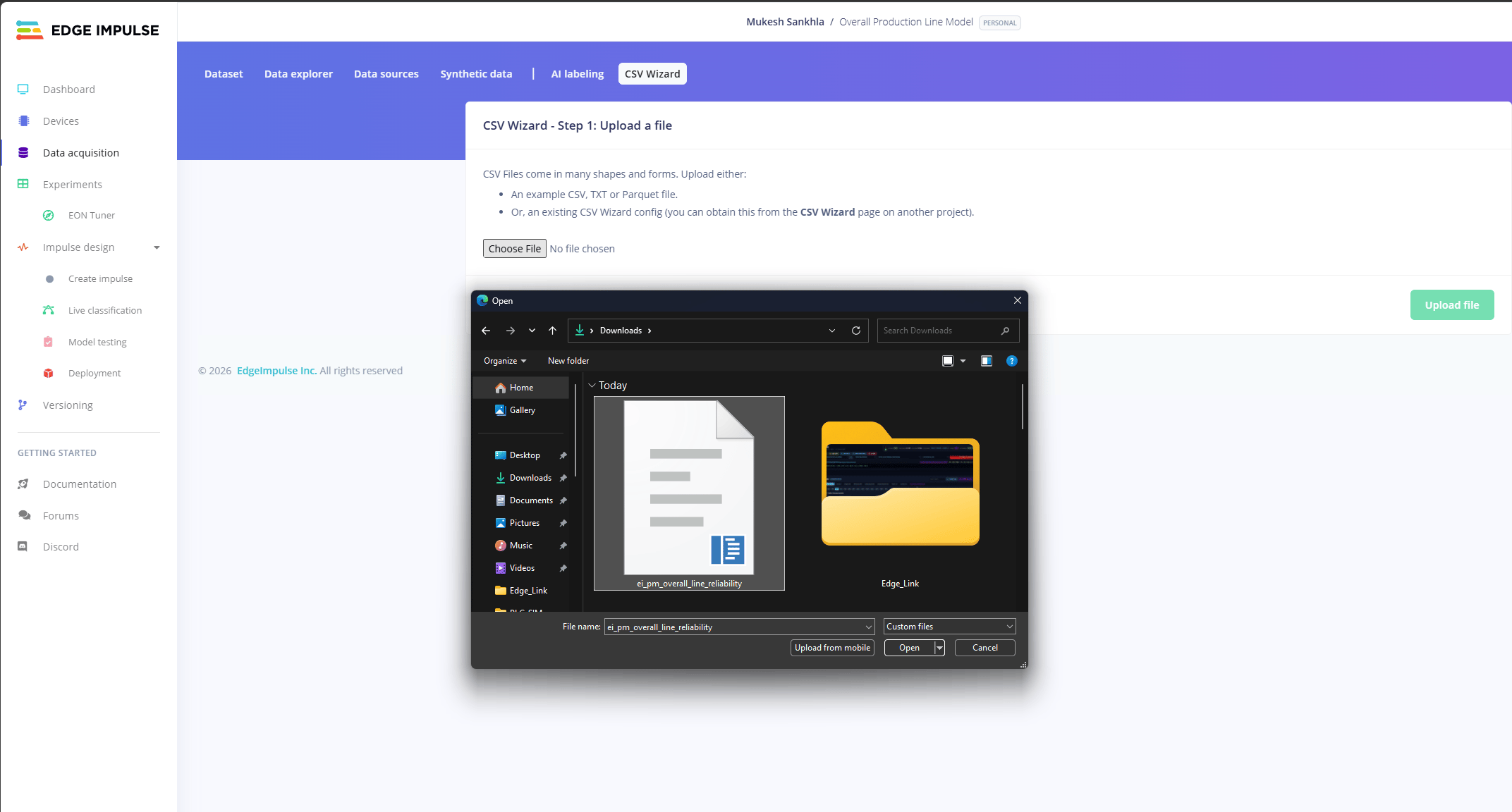
CSV Wizard tab and then upload CSV
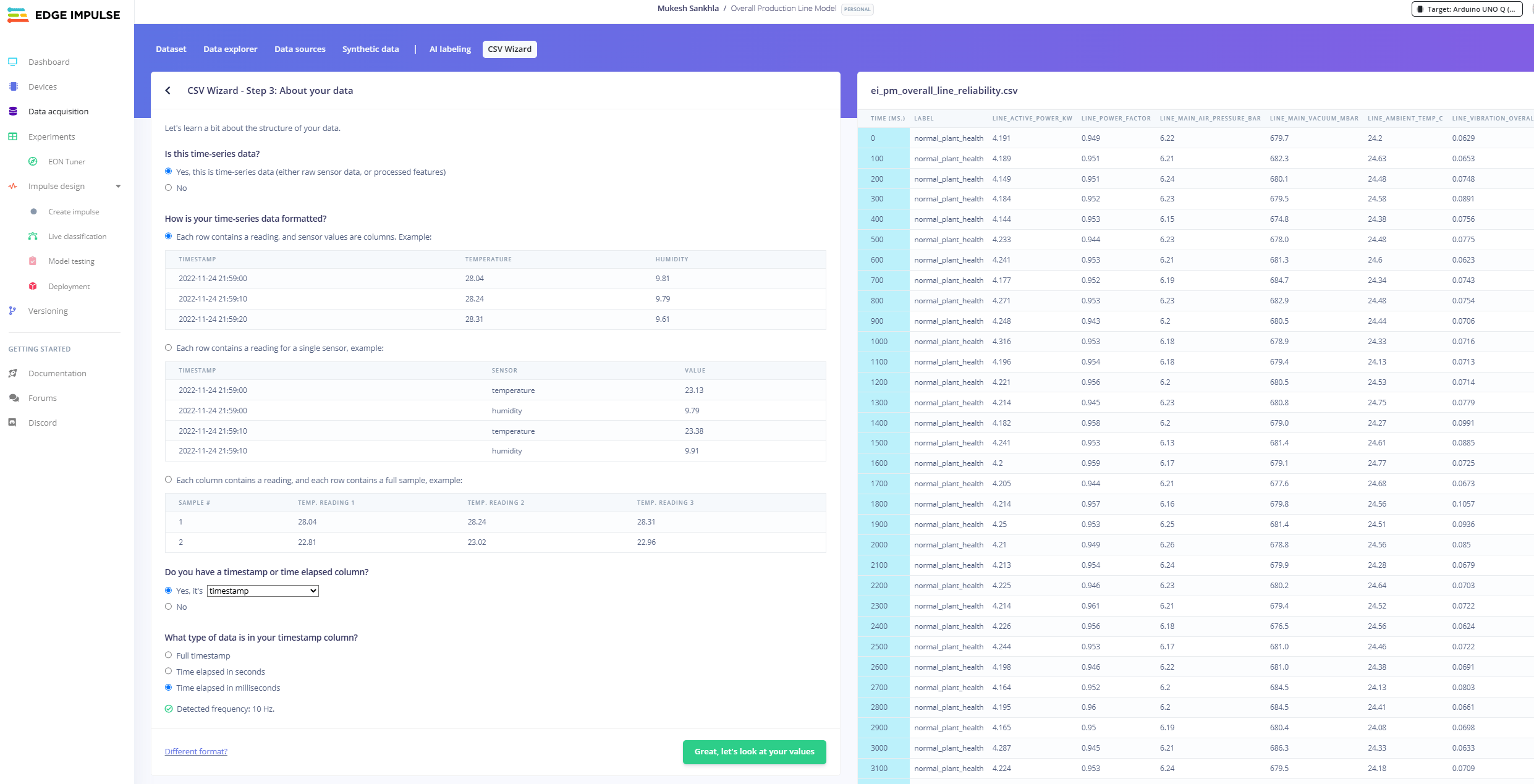
Configure the Time-Series Data
Edge Impulse will now ask how the CSV data is structured. For our predictive-maintenance dataset, select:- Is this time-series data?
- Yes, this is time-series data (either raw sensor data, or processed features)
- How is your time-series data formatted?
- Select: Each row contains a reading, and sensor values are columns.
- Do you have a timestamp or time elapsed column?
- Select: Yes
- What type of data is in your timestamp column?
- Select: Time elapsed in milliseconds
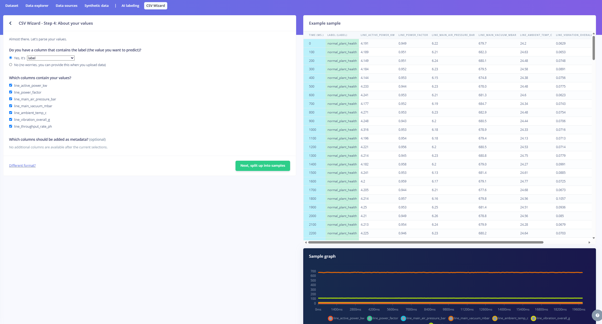
- Select: Do you have a column that contains the label (the value you want to predict)? Yes
- Select the column: label
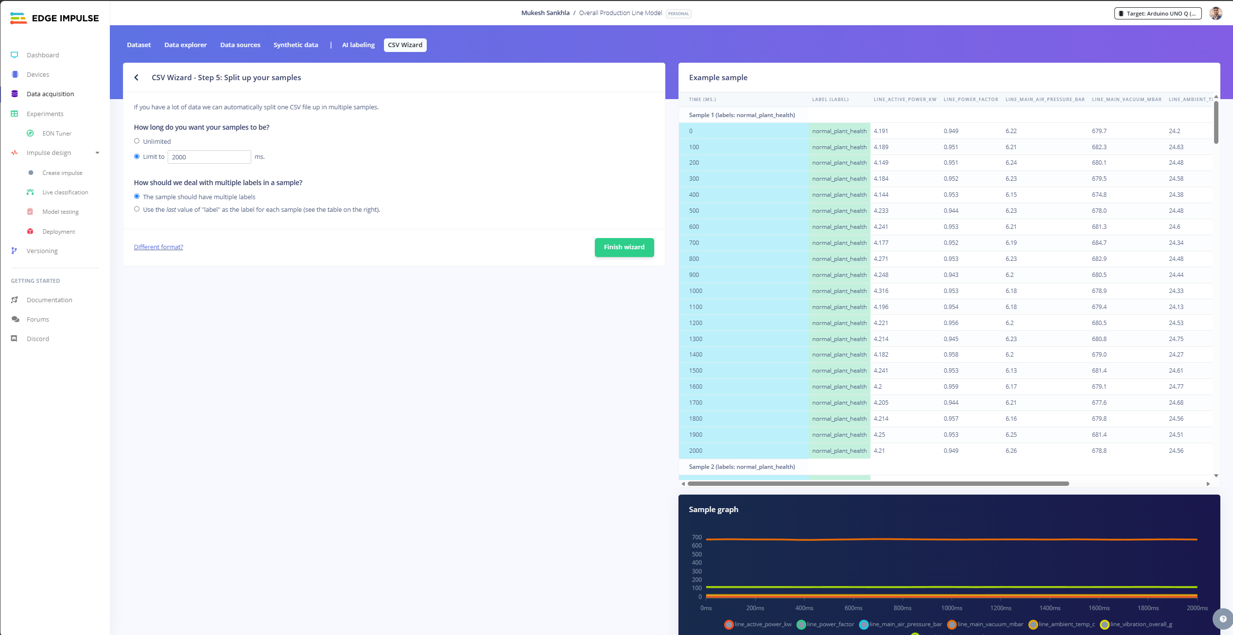
- How should we deal with multiple labels in a sample?
- Select: The sample should have multiple labels
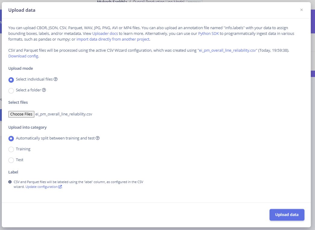
Upload the Dataset
After completing the CSV Wizard, click:Upload some data
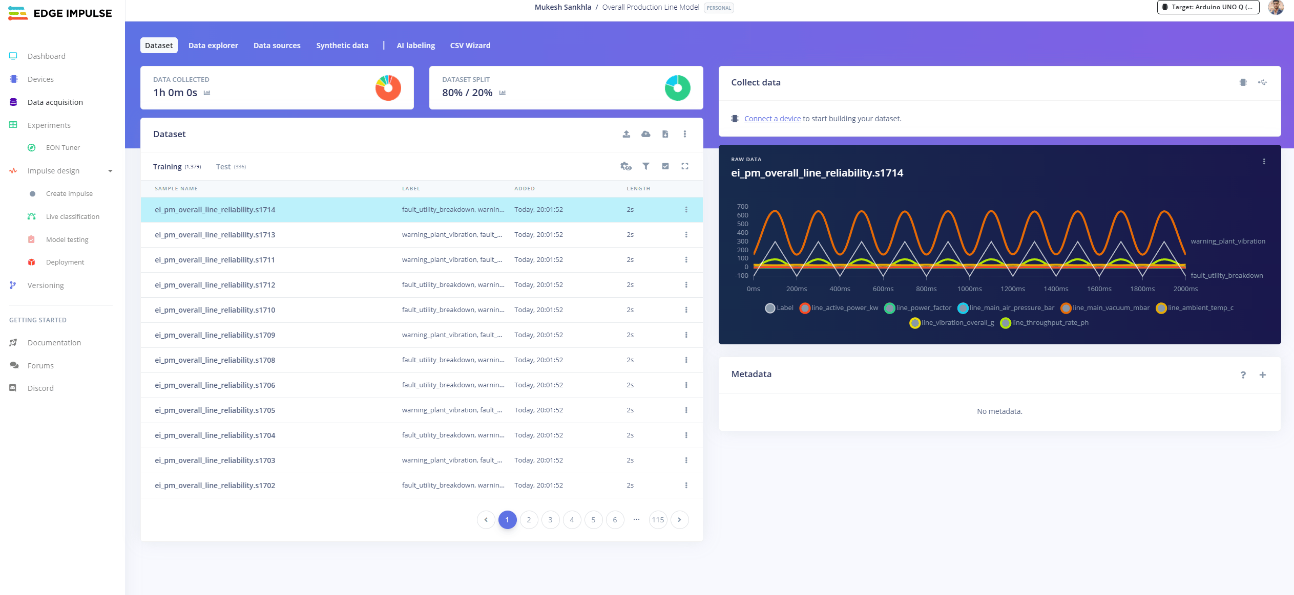
Create the Impulse
Now let’s create the Impulse for our predictive-maintenance model.- Go to
Create Impulse - Set the
Window sizeto 2000 ms. - Set the
Window increase (stride)to 2000 ms. - Under
Processing block, select Spectral Analysis. - Under
Learning block, select Classification and Anomaly Detection (K-Means). - Click
Save Impulse.
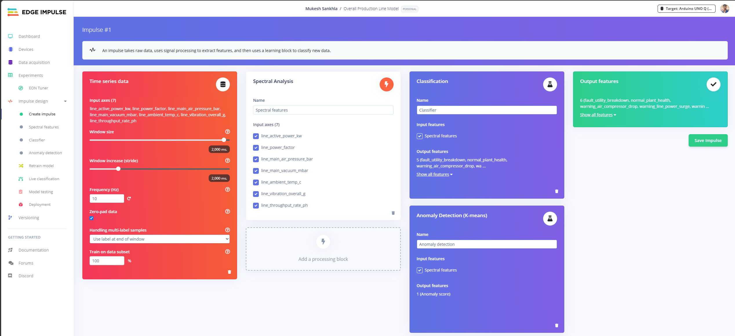
Generate Spectral Features
Go to Spectral Features.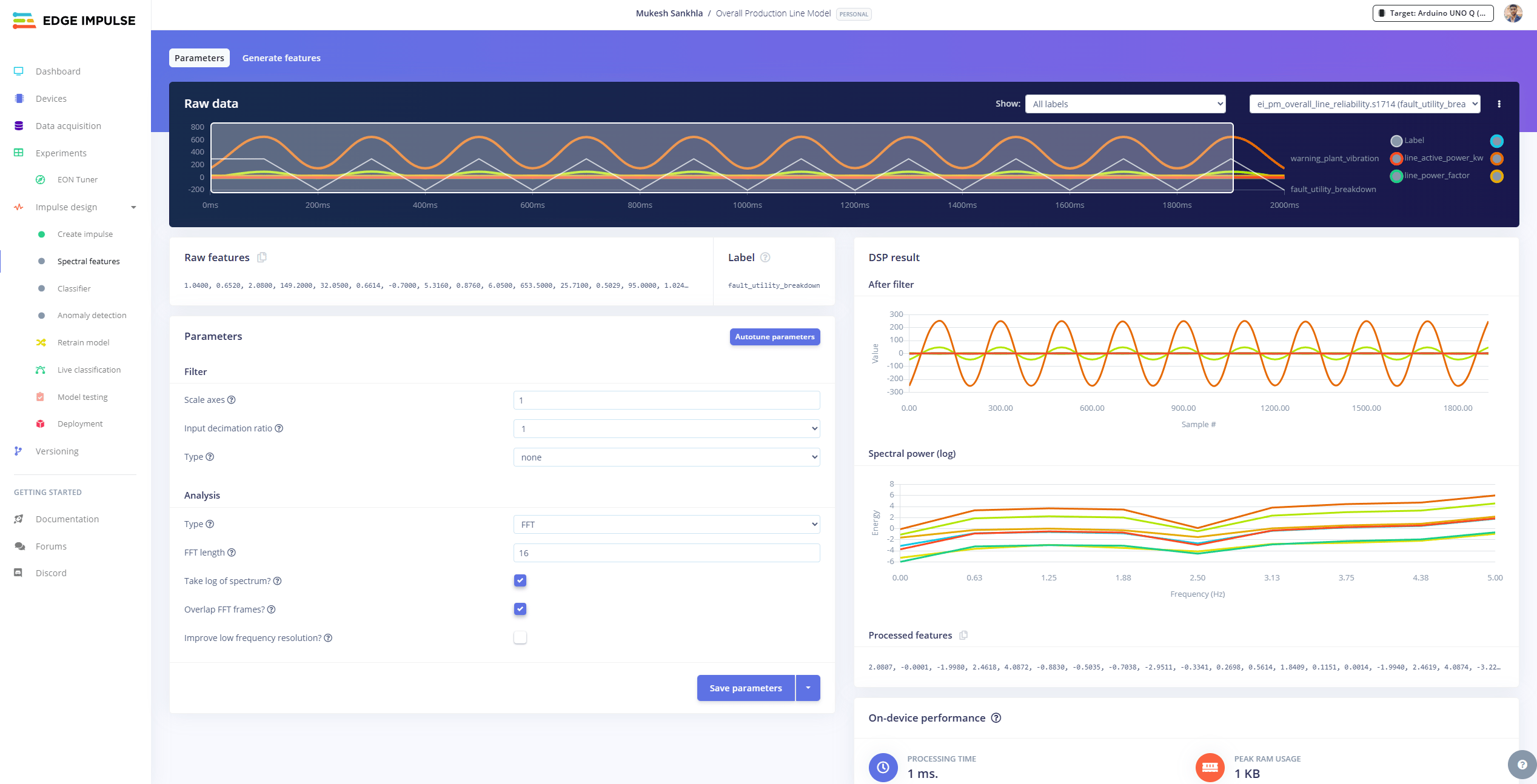
Save parameters
Next, go to Generate Features.
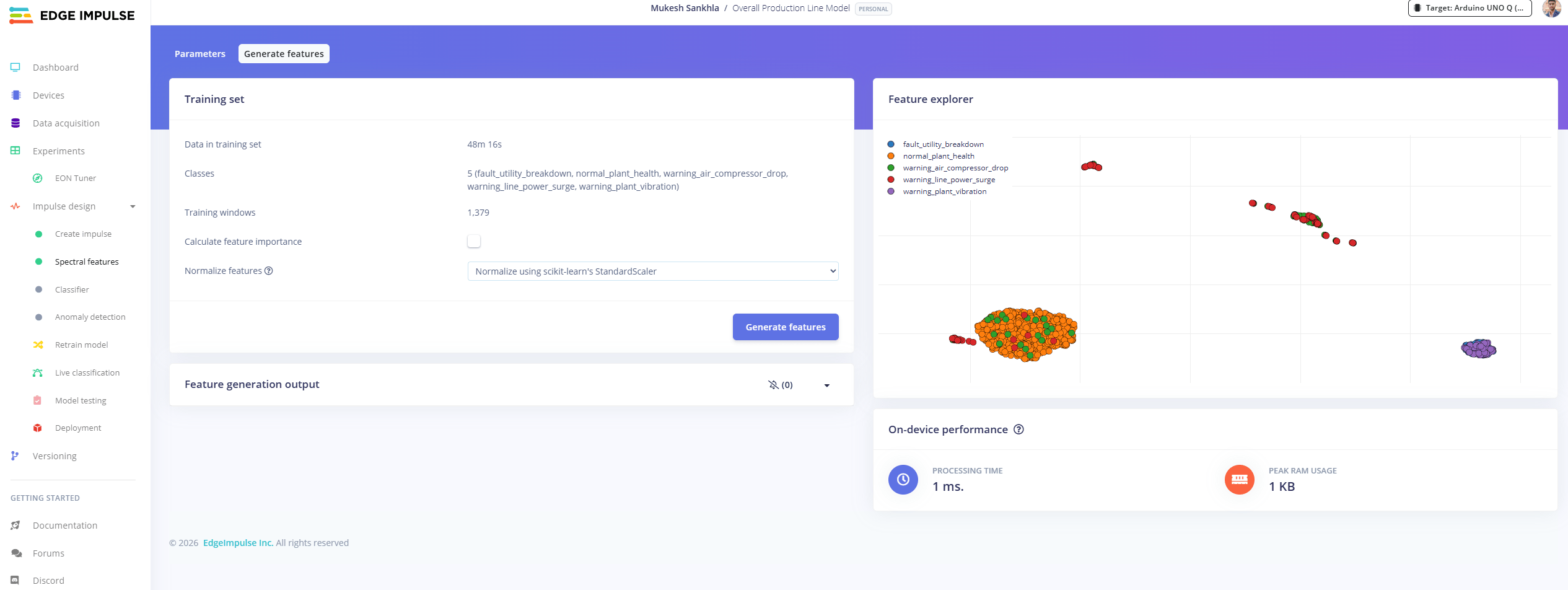
Normalize using the standard scaling method
Then click: Generate features
Edge Impulse will process all the samples in our dataset and generate the corresponding features. These generated features will now be used for the next step: training our Classification and Anomaly Detection models.
Train the Classification Model
Now go to the Classification page. Change the learning rate to 0.01, other settings at their default values and click:Save & Train
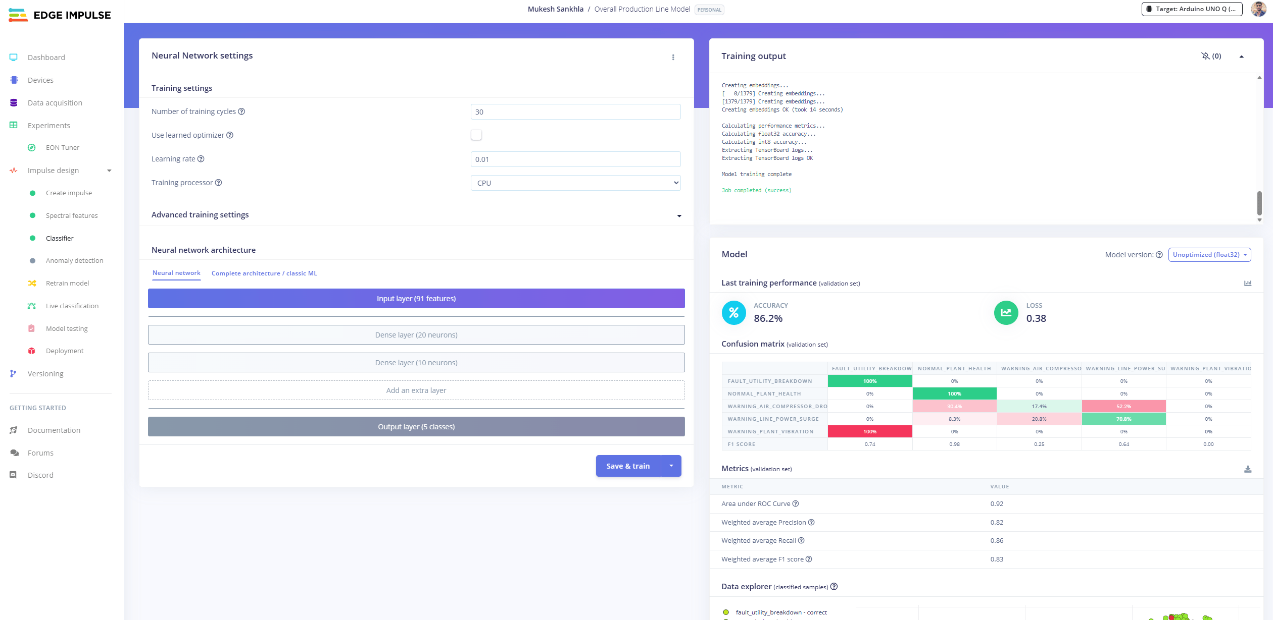
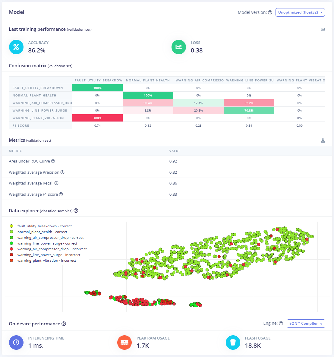
Example 1 - Overall Line Model
fault_utility_breakdown→ 100%normal_plant_health→ 100%warning_line_power_surge→ 70.8%
warning_air_compressor_drop is frequently classified as warning_line_power_surge.
This tells us that the features generated for these two conditions are relatively similar, so the model has difficulty separating them.
The other metrics are:
- AUC: 0.92
- Weighted Precision: 0.82
- Weighted Recall: 0.86
- Weighted F1: 0.83
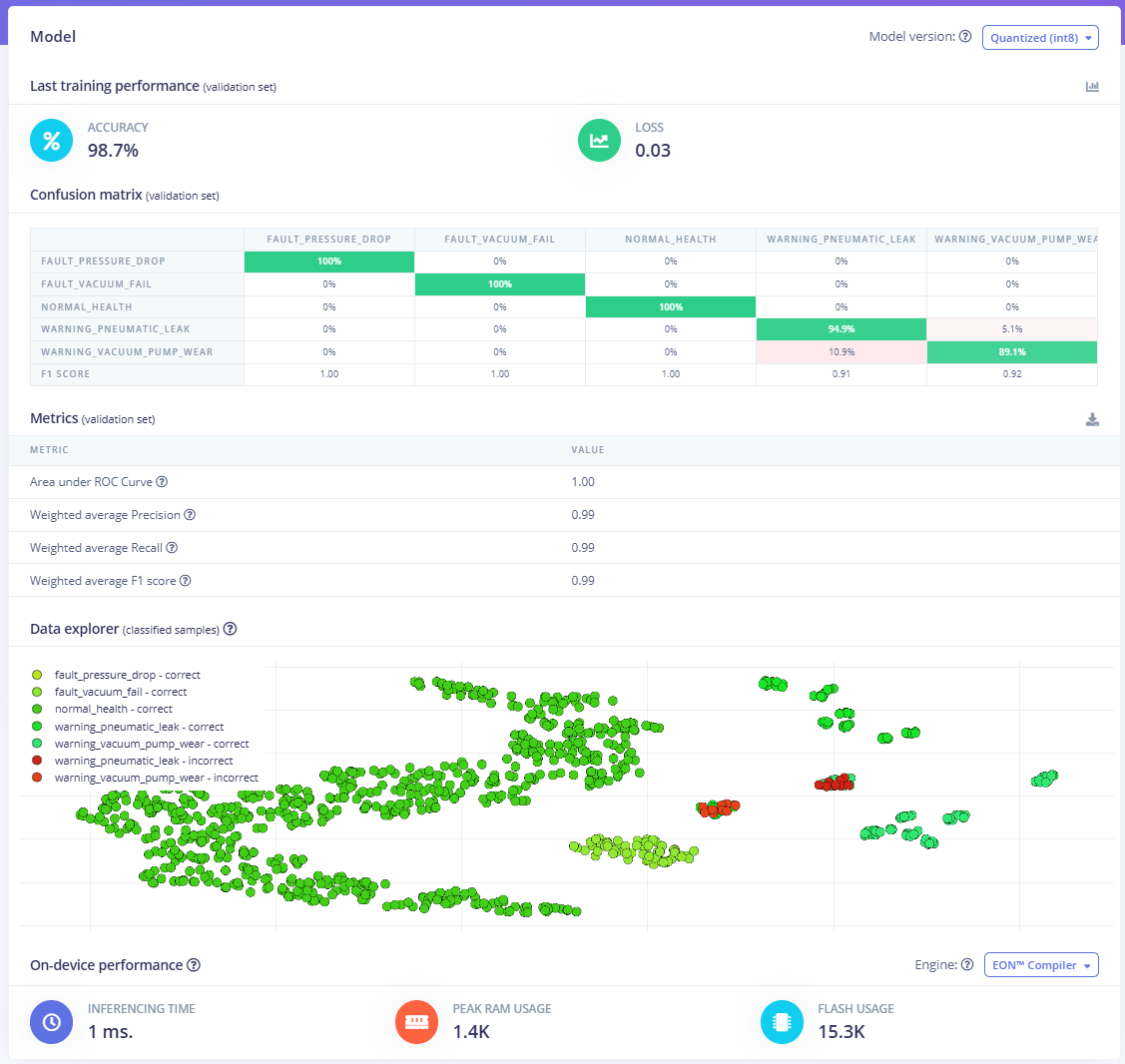
Example 2 - Station 4 Classification
- Validation Accuracy: 98.7%
- Loss: 0.03
fault_pressure_drop→ 100%fault_vacuum_fail→ 100%normal_health→ 100%warning_pneumatic_leak→ 94.9%warning_vacuum_pump_wear→ 89.1%
- AUC: 1.00
- Weighted Precision: 0.99
- Weighted Recall: 0.99
- Weighted F1: 0.99
- Inference time: 1 ms
- Peak RAM: 1.4 KB
- Flash usage: 15.3 KB
Why Do We Get Different Results?
- The two models don’t necessarily have the same difficulty.
- Different stations have different sensor characteristics and different fault conditions. Some conditions produce very distinctive patterns, while others may look very similar.
- For example, if two fault conditions produce almost identical vibration, temperature, current, or pressure patterns, the model will have a harder time distinguishing them.
- This is why dataset quality and feature selection are extremely important.
Let’s Experiment to Get Better Results
- Instead of simply accepting the first training result, we should experiment with the model configuration.
- There is no single configuration that is guaranteed to give the best result for every dataset.
- Try changing one parameter at a time and retrain the model.
Learning Rate
We used:0.01
Try different values and compare the results.
For example:
Window Size
We currently use:Window Stride
We currently use:2000 ms
Experiment with smaller strides if you want more overlapping training samples.
For example:
Spectral Analysis Parameters
- Don’t assume the default spectral configuration is always optimal.
- Experiment with the spectral feature configuration and observe the Feature Explorer.
- The goal is to get good separation between different machine-health classes.
- If two classes are heavily overlapping in the Feature Explorer, that is a sign that we may need better features or better data.
Most Important: Improve the Dataset
In my opinion, dataset quality is more important than simply tuning the learning rate. For every machine condition, try to generate enough representative data.Train the Anomaly Detection Model
Now let’s configure the Anomaly Detection model.- Go to the Anomaly Detection section.
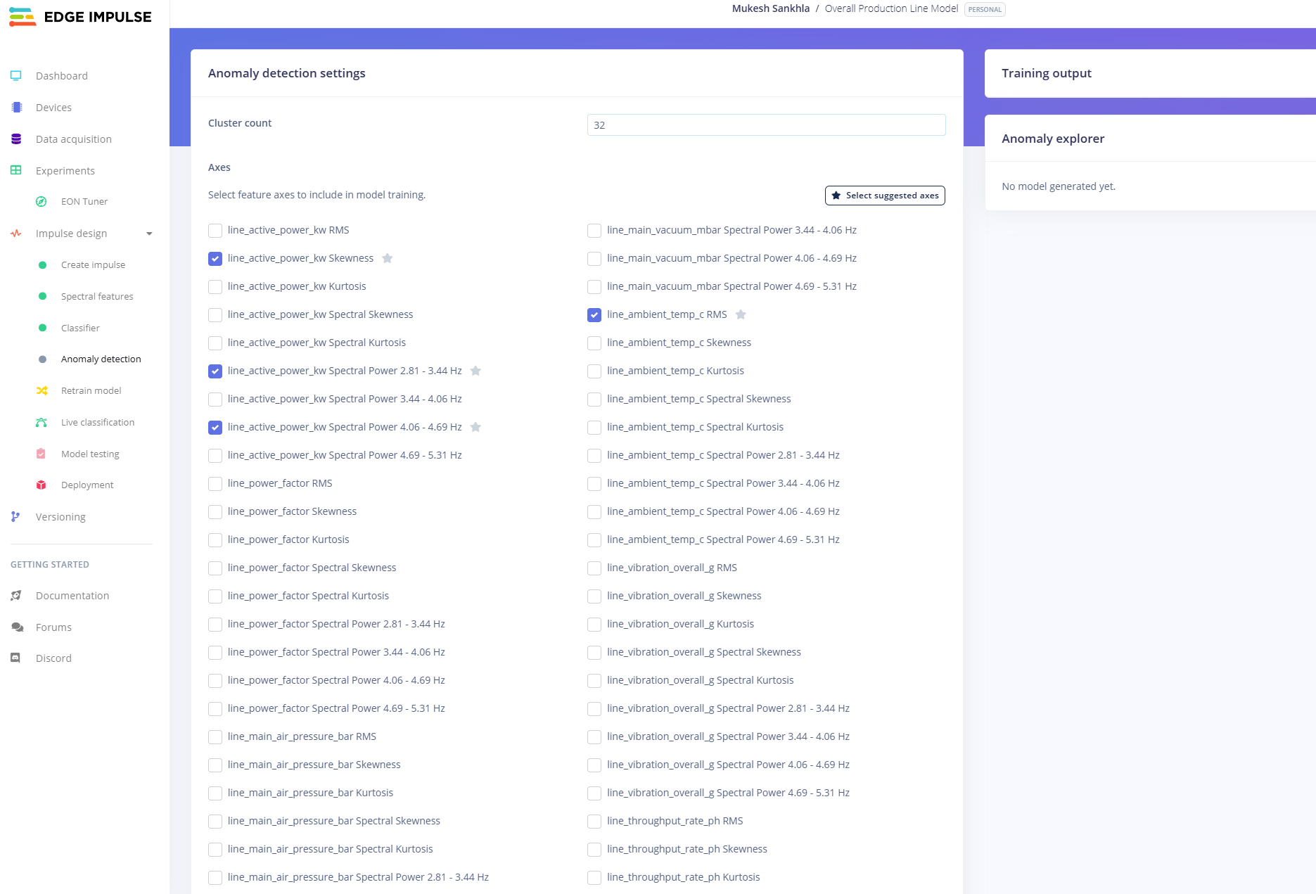
- Click Select suggested axes.
- Edge Impulse will automatically select the most suitable axes/features for the model.
- Click Save & Train.
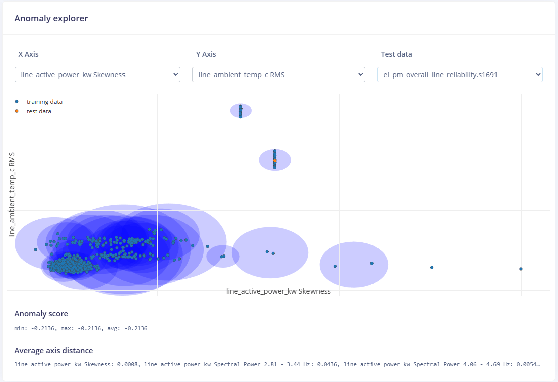
- The blue points/regions represent the training data and learned normal clusters.
- The orange points represent the test data.
- The selected axes are line_active_power_kw and line_ambient_temp_c with their extracted features.
- Points that stay close to the learned clusters are considered normal.
- Points that fall far outside the learned clusters can be identified as anomalies.
Deploy the Model to Arduino UNO Q
- Go to the Deployment page in Edge Impulse.
- Under Deployment Target, select Arduino UNO Q.
- Click Build.
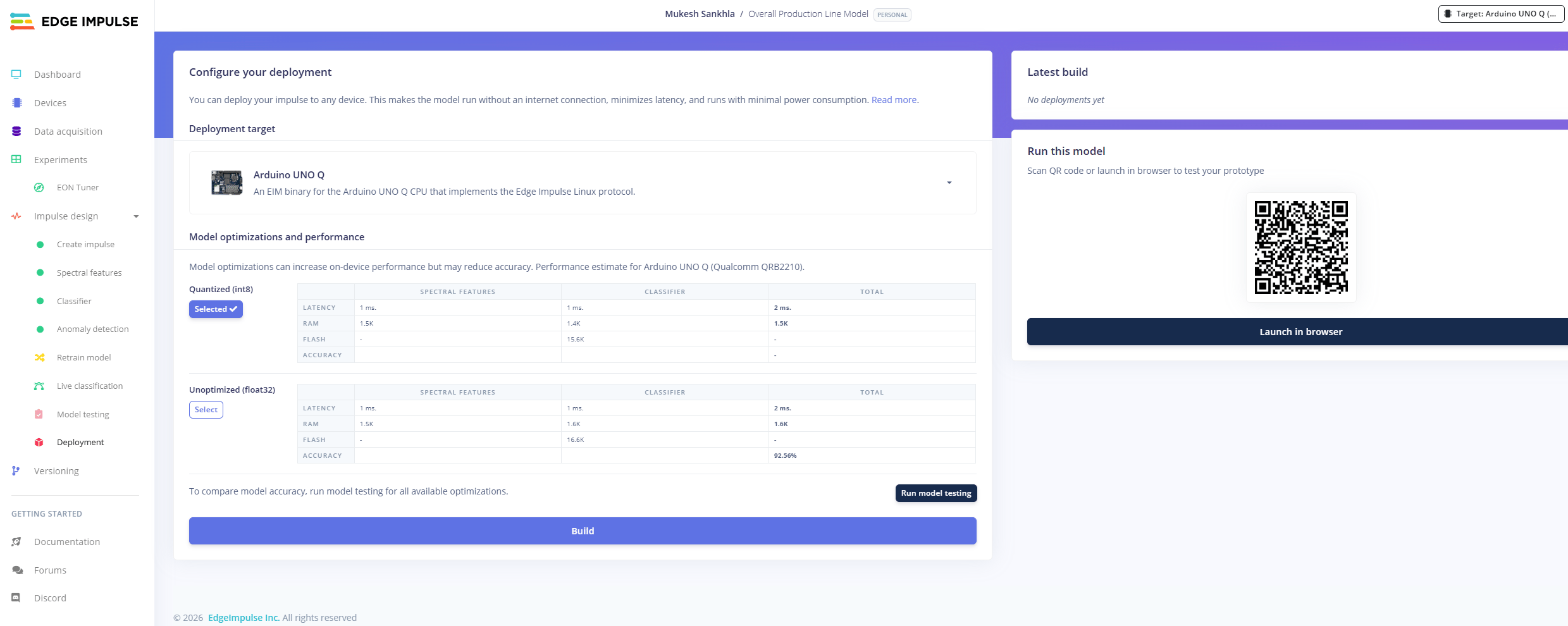
.eim model file, which can then be copied into the appropriate Arduino UNO Q / Edge Link application folder and configured for real-time Edge AI/ML inference directly on the UNO Q. Arduino’s current App Lab workflow also supports deploying custom Edge Impulse models to the UNO Q, with the model becoming available to the relevant AI brick after deployment.
The Edge Impulse models used in this project
- Overall Line Predictive Maintenance: Edge Impulse Project
- Station 1: Edge Impulse Project
- Station 2: Edge Impulse Project
- Station 3: Edge Impulse Project
- Station 4: Edge Impulse Project
- Station 5: Edge Impulse Project