

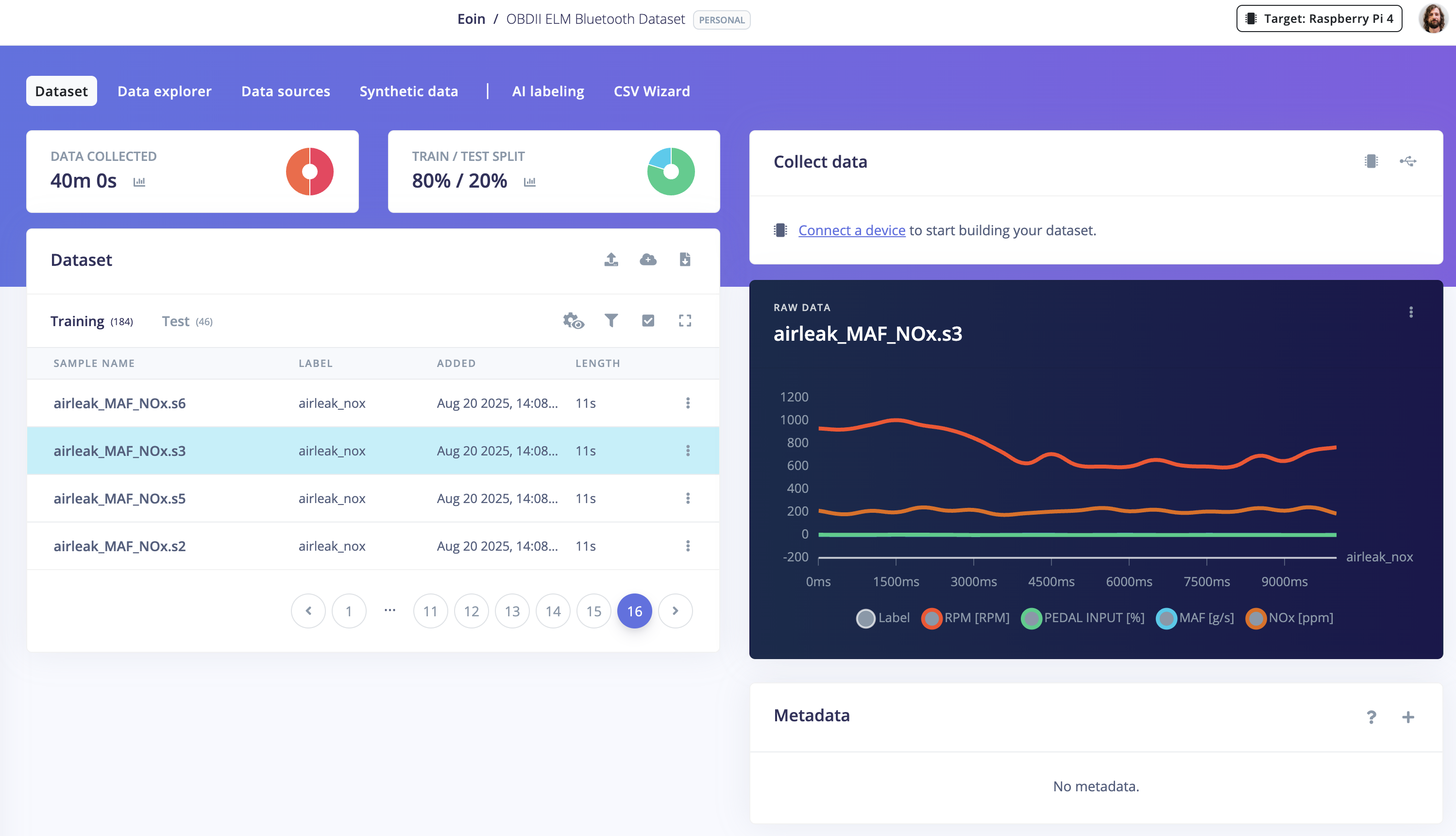
OBD formatted data
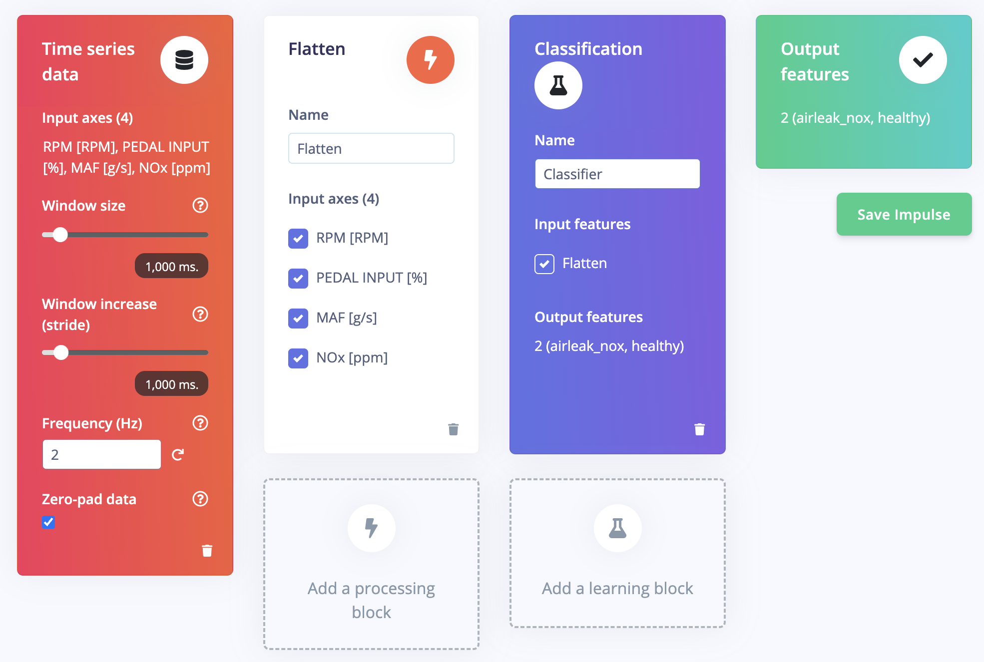
Impulse
Prerequisites
Before you begin, ensure you have the following:- An Edge Impulse account
- A compatible OBD-II adapter (e.g., ELM327)
- CSV of OBD-II data for healthy and unhealthy vehicle states
Take the sample CSV to get started or collect a sample from your OBD-II interface using your pi and the telemetry-obd project.
1. Problem overview
Goal: Detect an intake air leak from OBD-II signals by finding windows where NOx is disproportionately high relative to load (throttle / airflow / RPM).Signals we will use
We’ll use a minimal, interpretable set (more can be added later):- MAF [g/s] : proxy for air mass entering the engine (load).
- NOx [ppm] : emission outcome; rises with lean burn / mis-mix.
- PEDAL INPUT [%] : driver demand / load request.
- (Optional) RPM, MAP [kPa], Lambda, STFT/LTFT for context.
Leak hypothesis: With unmetered air, mixture trends lean > NOx is higher than expected for the same load.
Capture options
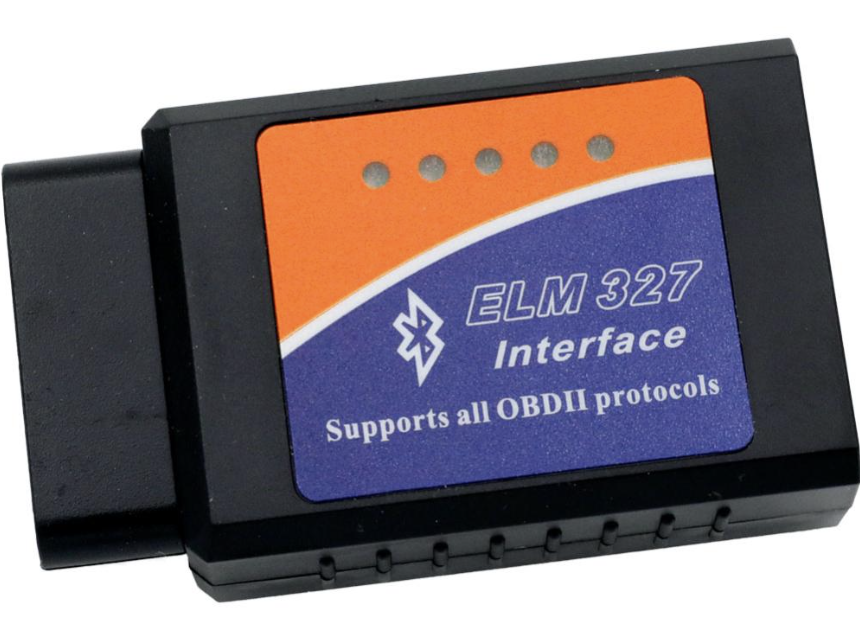
ELM327 USB or Bluetooth logger
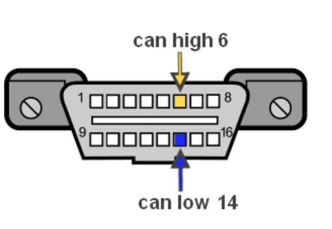
OBD-II connector pinout
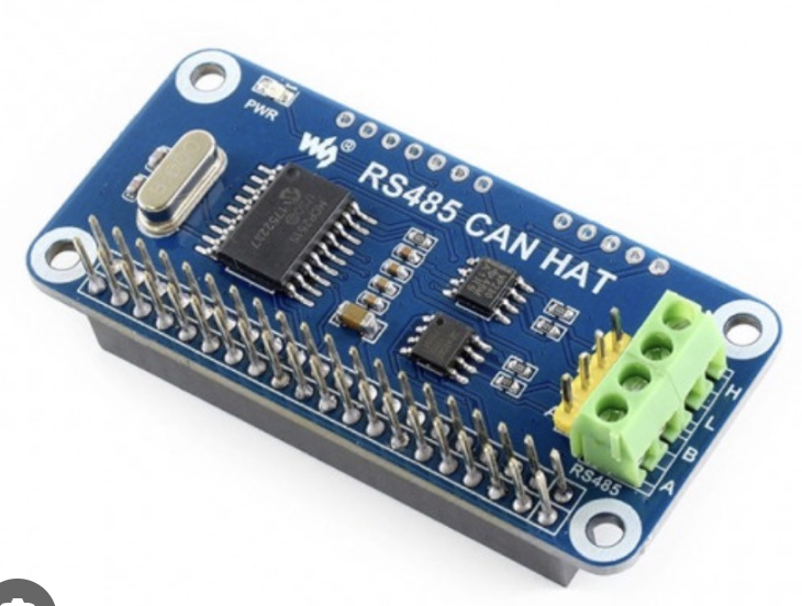
Pi Hat wiring
Safety note: Induce a small, reversible leak (loosen an intake boot or remove a tiny vacuum cap). unplug the airflow sensor (MAF/MAP) : this can trigger limp mode and confound data.
Data capture (reproducible method)
Capture- Sampling: 2 Hz (every 500 ms).
- Drive cycle: idle > gentle accelerations > light cruise > decel.
- Classes:
healthy: intact intake, warmed-up closed loop.airleak_nox: the same drive cycle with a small, controlled leak.
- Windows: 2000 ms window, 1000 ms step (overlapping).
- Duration target: ~10 min per class (balanced).
Window examples
Healthy window example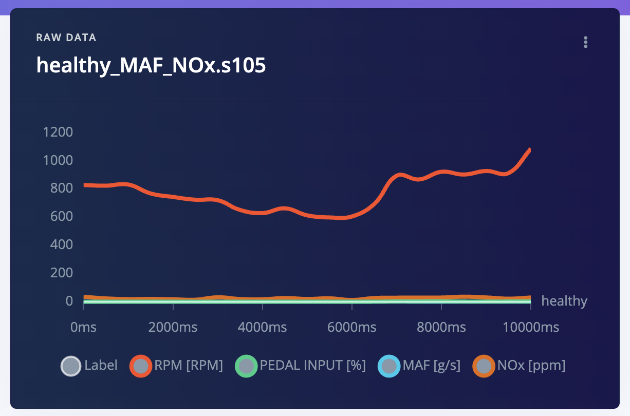
Healthy window (reference)
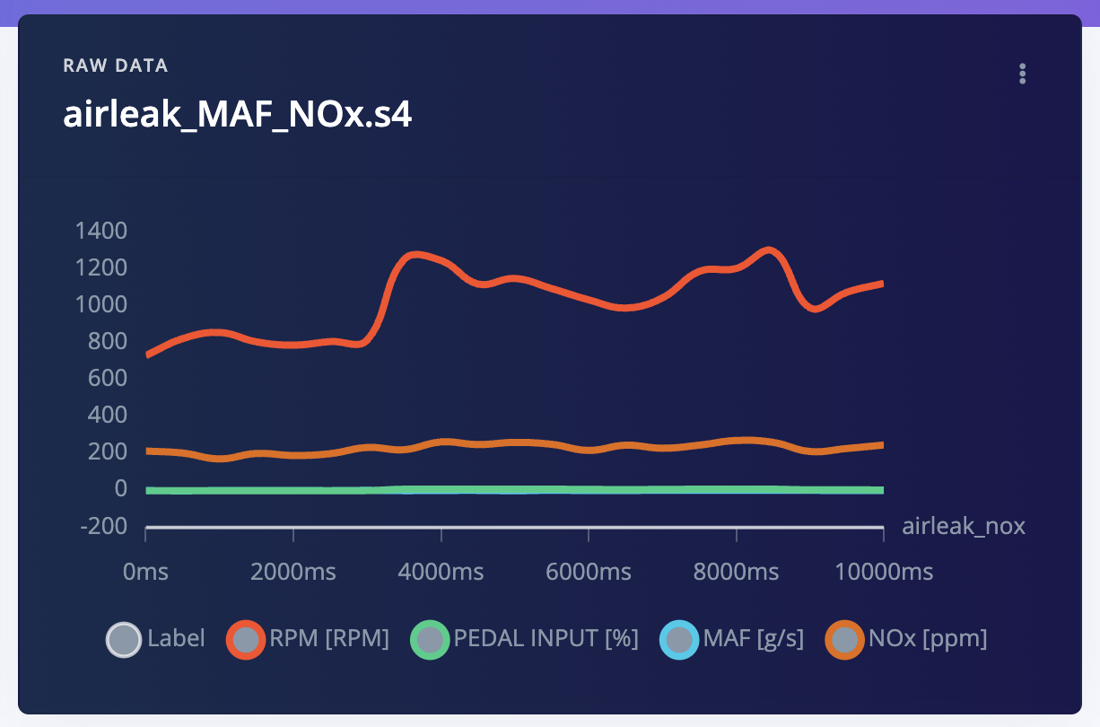
Air-leak window (high NOx vs load)
Simple, interpretable features
The ratios below are conceptual aids that explain the physics; you can compute them offline for analysis. In Studio, the Flatten block summarizes the raw channels directly. Over each 2 s window:nox_per_maf = NOx / max(MAF, 0.1)nox_per_throttle = NOx / max(throttle, 1)maf_per_rpm = MAF / max(RPM, 500)- Short-window mean and **slope ** for NOx and MAF
nox_per_maf and/or positive NOx slope at modest load are more likely air-leak.
With the signals defined, wiring settled, and an explicit labeling protocol, we can now build the model.
2. Prepare the CSV
The CSV Wizard expects:- A time column named
time (ms.)(milliseconds since the first sample) - One label column (here
fault_label) - One numeric column per OBD signal
Take the sample CSV to get started or collect a sample from your OBD-II interface using your pi and the telemetry-obd project.The CSVs for the sample project have the following headings:
3. Import with the CSV Wizard
- Open your project → Data acquisition → CSV Wizard
- Upload
n53_healthy_ei.csvandn53_faulty_ei.csv(or your own files) - Set Label column =
fault_labeland Time column =time (ms.) - Confirm sampling rate ≈ 2 Hz (every 500 ms)
- Finish import : the wizard converts each file into time-aligned samples
4. Windowing (time-series slicing)
Use windows long enough for trims/lambda to show trends:- Window size:
2000 ms - Window increase:
1000 ms
5. Create the impulse
- Go to Create impulse
- Input: your time-series window
- Processing block: Flatten (start simple)
- (Optional) add Spectral features for fast-changing channels (e.g.,
MAF [g/s],NOx [ppm]) - (Optional) enable Normalization if feature scales differ by ≥10×
- (Optional) add Spectral features for fast-changing channels (e.g.,
- Learning block: Classification (Keras)
Start with Flatten only. If accuracy plateaus, add Spectral features as a second block.
6. Generate features
Open Generate features and run on all samples.Use Feature explorer to verify clusters separate (healthy vs. fault).
7. Train the classifier
In Classification (Keras):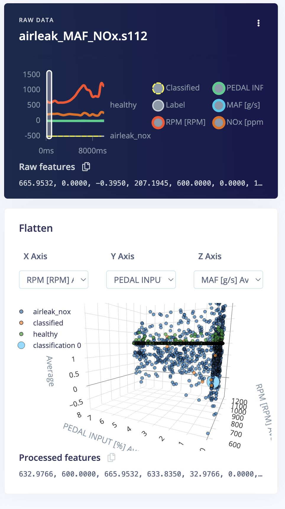
Classification
- Dense 128 (ReLU) → Dropout 0.20
- Dense 64 (ReLU)
- Dense N_classes (Softmax)
- Split: 70/30 train/validation
- Epochs: 50–100
- Batch size: 32
- Enable Class weighting if classes are imbalanced
Target: ≥ 95% precision/recall per class on the validation set.
8. Evaluate the model
- Confusion matrix: identify misclassifications (e.g., healthy ↔ fault)
- Feature explorer: confirm separation (trims/lambda/MAF/MAP)
- If one sensor dominates (e.g., only NOx), add more context:
- STFT/LTFT (fuel trims)
- Lambda (bank1/2)
- Ratios (e.g.,
maf_per_rpm,map_per_throttle)
9. Deploy
Open Deploy and choose your target:- Linux/Aarch64 (Raspberry Pi4)
Scripts
We have created a short script that will play back a recording of the CSV file and simulate real-time classification of the OBD-II signals. This allows us to test the model’s performance in a controlled environment before deploying it to a live vehicle, scripts and instructions are available from the public repository. obd automotive data Run the collection script to log data from your ELM327:Conclusion
In this tutorial, we explored how to collect OBD-II data from vehicles using both Bluetooth adapters and direct CAN bus connections, then trained and deployed a classifier that flags an intake air leak from the relationship between NOx and engine load. This workflow generalizes to other vehicle faults (misfire, EGR, sensor bias) and industrial CAN signals.Related work
If you use this tutorial or build on the approach described here, please cite the following paper:E. Jordan, M. Serrano, A. Gyrard, E. Song, T. Roth and D. Wollman, “Semantics for Enhancing Communications- and Edge-Intelligence-enabled Smart Sensors: A Practical Use Case in Federated Automotive Diagnostics,” IECON 2024 - 50th Annual Conference of the IEEE Industrial Electronics Society, Chicago, IL, USA, 2024, pp. 1-6, doi: 10.1109/IECON55916.2024.10905565.