1. Prerequisites
For this tutorial, you’ll need a supported device. Alternatively, use the either Data forwarder or Edge Impulse for Linux SDK to collect data from any other development board, or your mobile phone. If your device is connected (green dot) under Devices in the studio you can proceed: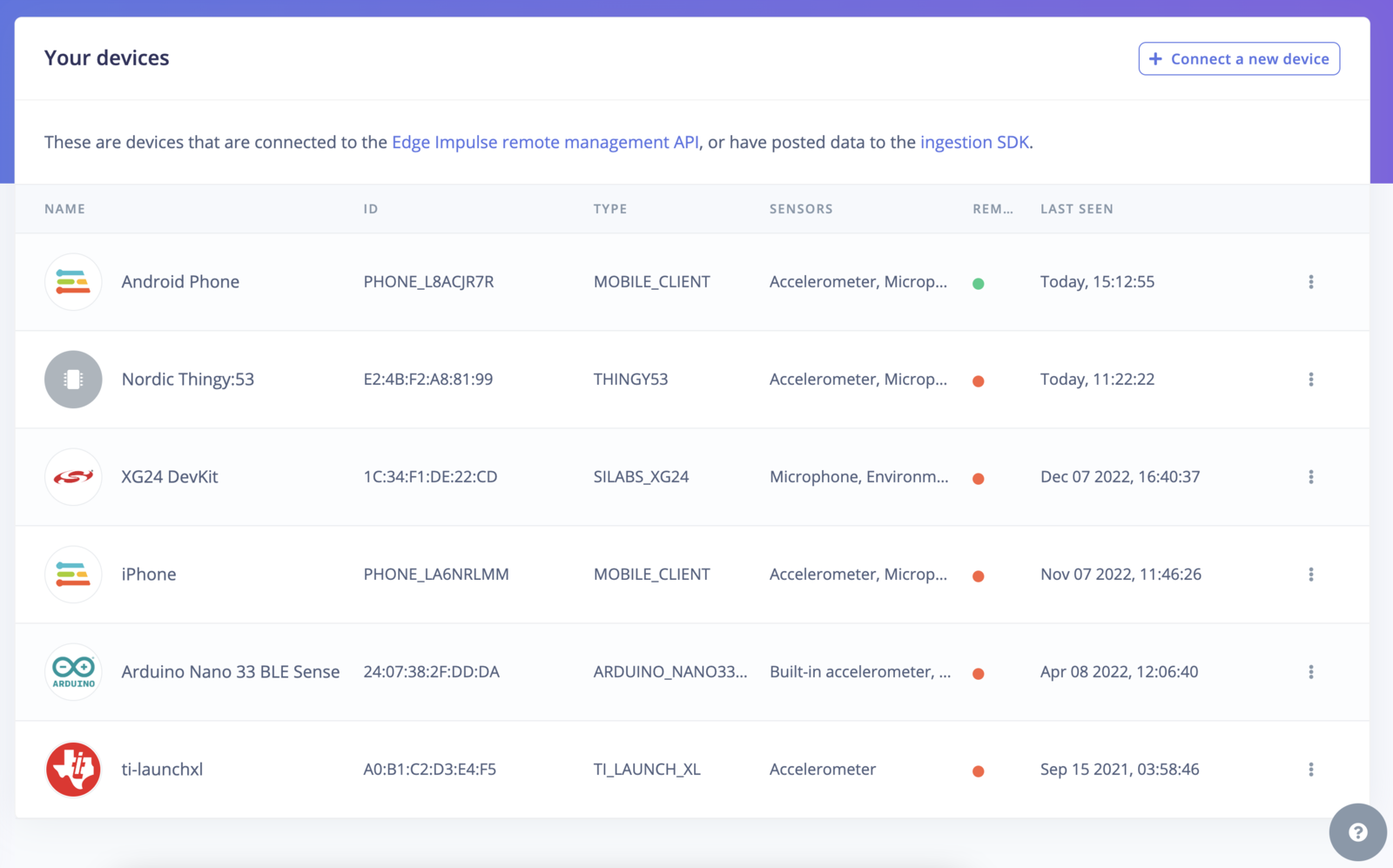
Devices tab with the device connected to the remote management interface.
2. Collecting your first data
With your device connected, we can collect some data. In the studio go to the Data acquisition tab. This is the place where all your raw data is stored, and - if your device is connected to the remote management API - where you can start sampling new data. Under Record new data, select your device, set the label toupdown, the sample length to 10000, the sensor to Built-in accelerometer and the frequency to 62.5Hz. This indicates that you want to record data for 10 seconds, and label the recorded data as updown. You can later edit these labels if needed.
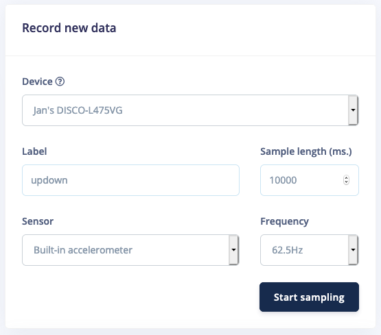
Record new data screen.
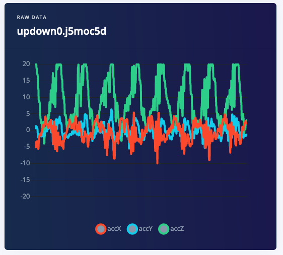
Updown movement recorded from the accelerometer.
- Idle - just sitting on your desk while you’re working.
- Snake - moving the device over your desk as a snake.
- Wave - waving the device from left to right.
- Updown - moving the device up and down.
3. Designing an impulse
With the training set in place, you can design an impulse. An impulse takes the raw data, slices it up in smaller windows, uses signal processing blocks to extract features, and then uses a learning block to classify new data. Signal processing blocks always return the same values for the same input and are used to make raw data easier to process, while learning blocks learn from past experiences. For this tutorial we’ll use the ‘Spectral analysis’ signal processing block. This block applies a filter, performs spectral analysis on the signal, and extracts frequency and spectral power data. Then we’ll use a ‘Neural Network’ learning block, that takes these spectral features and learns to distinguish between the four (idle, snake, wave, updown) classes. In the studio go to Create impulse, set the window size to2000 (you can click on the 2000 ms. text to enter an exact value), the window increase to 80, and add the ‘Spectral Analysis’ and ‘Classification (Keras)’ blocks. Then click Save impulse.
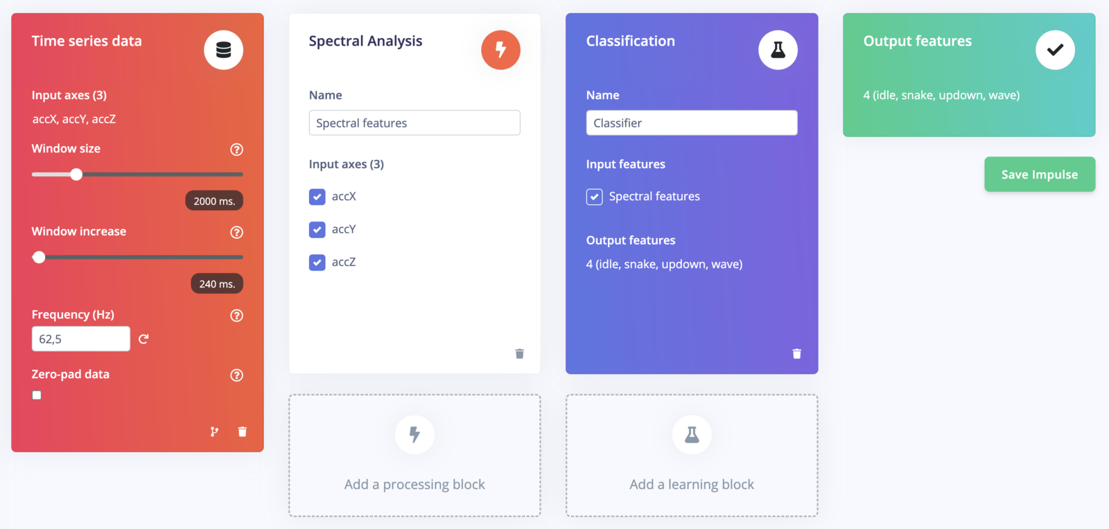
First impulse, with one processing block and one learning block.
Configuring the spectral analysis block
To configure your signal processing block, click Spectral features in the menu on the left. This will show you the raw data on top of the screen (you can select other files via the drop down menu), and the results of the signal processing through graphs on the right. For the spectral features block you’ll see the following graphs:- Filter response - If you have chosen a filter (with non zero order), this will show you the response across frequencies. That is, it will show you how much each frequency will be attenuated.
- After filter - the signal after applying the filter. This will remove noise.
- Spectral power - the frequencies at which the signal is repeating (e.g. making one wave movement per second will show a peak at 1 Hz).
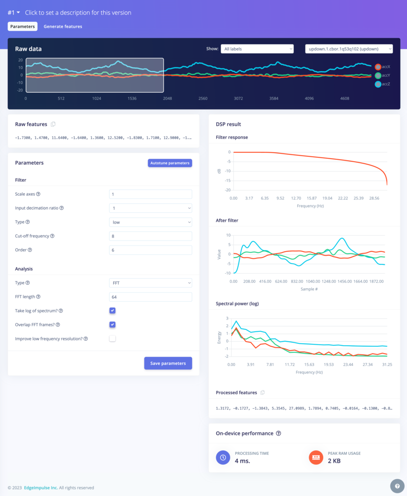
Spectral features parameters
- Split all raw data up in windows (based on the window size and the window increase).
- Apply the spectral features block on all these windows.
- Calculate feature importance. We will use this later to set up the anomaly detection.
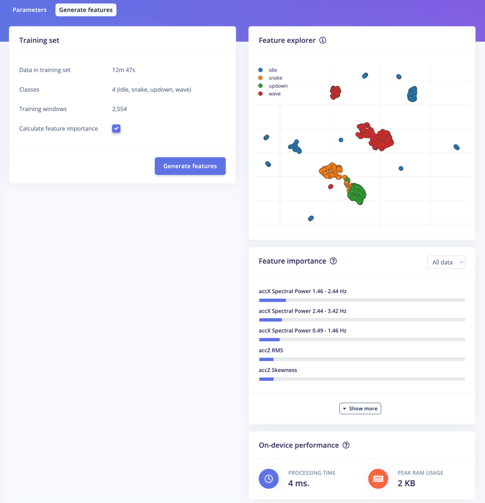
Spectral features - Generate features
Configuring the neural network
With all data processed it’s time to start training a neural network. Neural networks are a set of algorithms, modeled loosely after the human brain, that are designed to recognize patterns. The network that we’re training here will take the signal processing data as an input, and try to map this to one of the four classes. So how does a neural network know what to predict? A neural network consists of layers of neurons, all interconnected, and each connection has a weight. One such neuron in the input layer would be the height of the first peak of the X-axis (from the signal processing block); and one such neuron in the output layer would bewave (one the classes). When defining the neural network all these connections are initialized randomly, and thus the neural network will make random predictions. During training, we then take all the raw data, ask the network to make a prediction, and then make tiny alterations to the weights depending on the outcome (this is why labeling raw data is important).
This way, after a lot of iterations, the neural network learns; and will eventually become much better at predicting new data. Let’s try this out by clicking on NN Classifier in the menu.
1. This will limit training to a single iteration. And then click Start training.
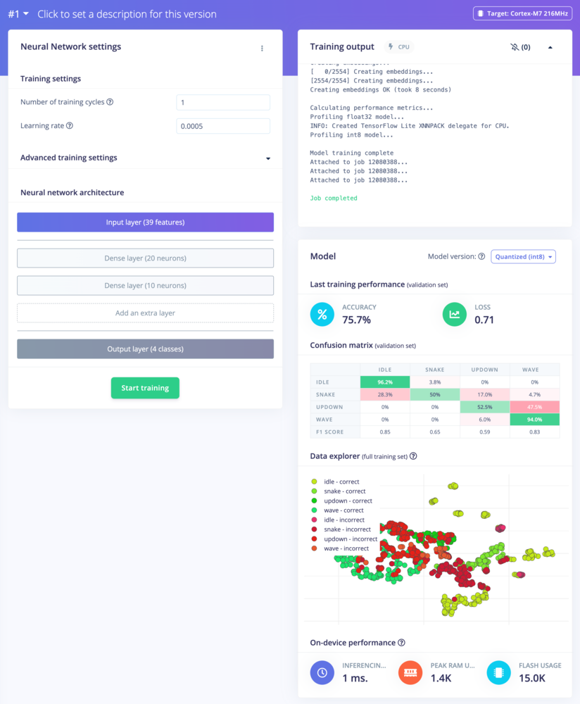
Training performance after a single iteration. On the top-right, is a summary of the accuracy of the network, and in the middle, a confusion matrix. This matrix shows when the network made correct and incorrect decisions. You see that idle is relatively easy to predict. Why do you think this is?
2 and you’ll see performance go up. Finally, change ‘Number of training cycles’ to 30 and let the training finish.
You’ve just trained your first neural networks!
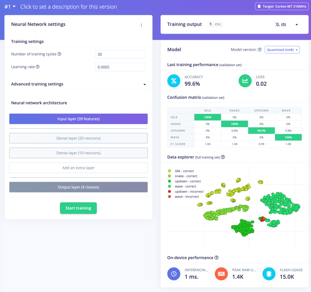
Neural network trained with 30 epochs
4. Classifying new data
From the statistics in the previous step we know that the model works against our training data, but how well would the network perform on new data? Click on Live classification in the menu to find out. Your device should (just like in step 2) show as online under ‘Classify new data’. Set the ‘Sample length’ to10000 (10 seconds), click Start sampling and start doing movements. Afterward, you’ll get a full report on what the network thought you did.
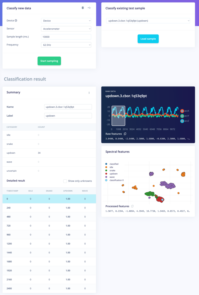
Classification result. Showing the conclusions, the raw data and processed features in one overview.
- There is not enough data. Neural networks need to learn patterns in data sets, and the more data the better.
- The data does not look like other data the network has seen before. This is common when someone uses the device in a way that you didn’t add to the test set. You can add the current file to the test set by clicking
⋮, then selecting Move to training set. Make sure to update the label under ‘Data acquisition’ before training. - The model has not been trained enough. Up the number of epochs to
200and see if performance increases (the classified file is stored, and you can load it through ‘Classify existing validation sample’). - The model is overfitting and thus performs poorly on new data. Try reducing the learning rate or add more data.
- The neural network architecture is not a great fit for your data. Play with the number of layers and neurons and see if performance improves.
5. Anomaly detection
Neural networks are great, but they have one big flaw. They’re terrible at dealing with data they have never seen before (like a new gesture). Neural networks cannot judge this, as they are only aware of the training data. If you give it something unlike anything it has seen before it’ll still classify as one of the four classes. Let’s look at how this works in practice. Go to ‘Live classification’ and record some new data, but now vividly shake your device. Take a look and see how the network will predict something regardless. So, how can we do better? If you look at the feature explorer, you should be able to visually separate the classified data from the training data. We can use this to our advantage by training a new (second) network that creates clusters around data that we have seen before, and compares incoming data against these clusters. If the distance from a cluster is too large you can flag the sample as an anomaly, and not trust the neural network.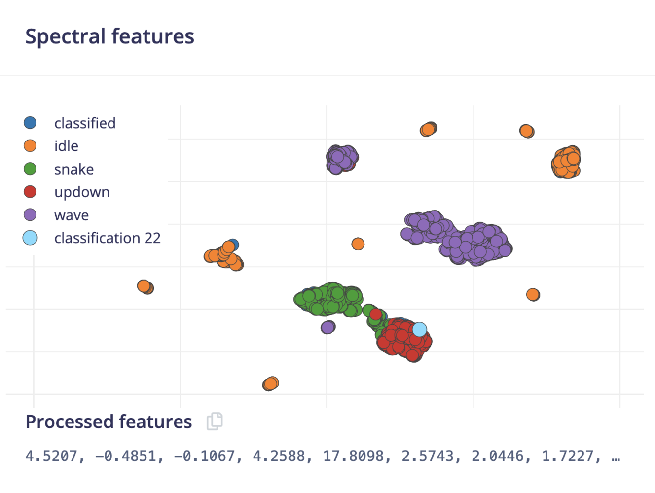
Shake data is easily separated from the training data.
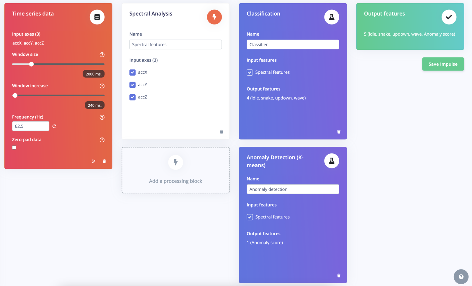
Add anomaly detection block to Create impulse tab
- The number of clusters. Here use
32. - The axes that we want to select during clustering. Click on the Select suggested axes button to harness the results of the feature importance output. Alternatively, the data separates well on the accX RMS, accY RMS and accZ RMS axes, you can also include these axes.
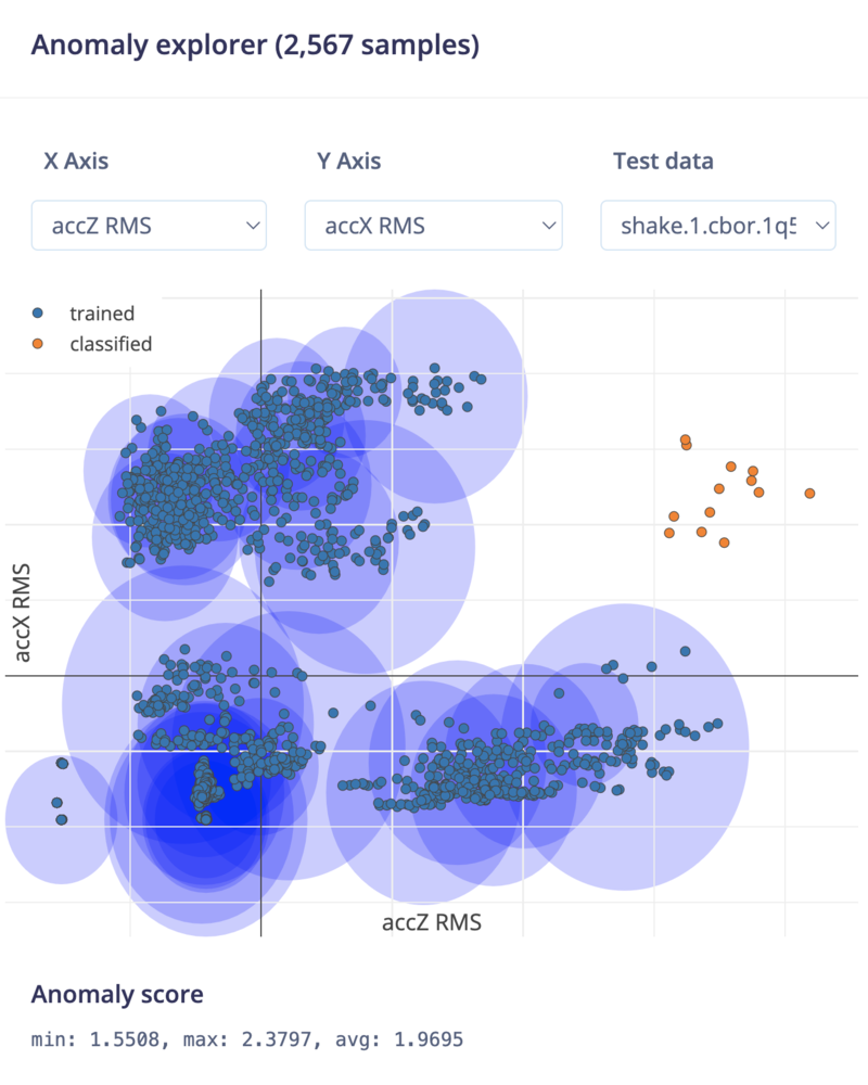
Known clusters in blue, the shake data in orange. It's clearly outside of any known clusters and can thus be tagged as an anomaly.
6. Deploying back to device
With the impulse designed, trained and verified you can deploy this model back to your device. This makes the model run without an internet connection, minimizes latency, and runs with minimum power consumption. Edge Impulse can package up the complete impulse - including the signal processing code, neural network weights, and classification code - up in a single C++ library that you can include in your embedded software.Flashing the device
When you click the Build button, you’ll see a pop-up with text and video instructions on how to deploy the binary to your particular device. Follow these instructions. Once you are done, we are ready to test your impulse out.Running the model on the device
We can connect to the board’s newly flashed firmware over serial. Open a terminal and run: