Building custom processing blocks

Extracting meaningful features from your data is crucial to building small and reliable machine learning models, and in Edge Impulse this is done through processing blocks. We ship a number of processing blocks for common sensor data (such as vibration and audio), but they might not be suitable for all applications. Perhaps you have a very specific sensor, want to apply custom filters, or are implementing the latest research in digital signal processing. In this tutorial you'll learn how to support these use cases by adding custom processing blocks to the studio.

There is also a complete video covering how to implement your custom DSP block:

Prerequisites

Make sure you follow the Continuous motion recognition tutorial, and have a trained impulse.

Development flow

This tutorial shows you the development flow of building custom processing blocks, and requires you to run the processing block on your own machine or server. Enterprise customers can share processing blocks within their organization, and run these on our infrastructure. See Hosting custom DSP blocks for more details.

1. Building your first custom processing block

Processing blocks take data and configuration parameters in, and return features and visualizations like graphs or images. To communicate to custom processing blocks, Edge Impulse studio will make HTTP calls to the block, and then use the response both in the UI, while generating features, or when training a machine learning model. Thus, to load a custom processing block we'll need to run a small server that responds to these HTTP calls. You can write this in any language, but we have created an example in Python. To load this example, open a terminal and run: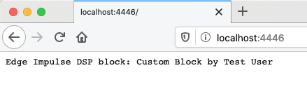

$ git clone https://github.com/edgeimpulse/example-custom-processing-block-python

This creates a copy of the example project locally. Then, you can run the example either through Docker or locally via:

Docker

$ docker build -t custom-blocks-demo .
$ docker run -p 4446:4446 -it --rm custom-blocks-demo

Locally

$ pip3 install -r requirements-blocks.txt
$ python3 dsp-server.py

Then go to http://localhost:4446 and you should be shown some information about the block.

Running your first custom block locally

Exposing the processing block to the world

As this block is running locally the studio cannot reach the block. To resolve this we can use ngrok which can make a local port accessible from a public URL. After you've finished development you can move the processing block to a server with a publicly accessible address (or run it on our infrastructure through your enterprise account). To set up a tunnel:

1. Sign up for ngrok.

2. Install the ngrok binary for your platform.

3. Get a URL to access the processing block from the outside world via:

$ ngrok http 4446
# or
$ ./ngrok http 4446

This yields a public URL for your block under Forwarding. Note down the address that includes https://.

Session Status                online
Account                       Edge Impulse (Plan: Free)
Version                       2.3.35
Region                        United States (us)
Web Interface                 http://127.0.0.1:4040
Forwarding                    http://4d48dca5.ngrok.io -> http://localhost:4446
Forwarding                    https://4d48dca5.ngrok.io -> http://localhost:4446

Adding the custom block to Edge Impulse

Now that the custom processing block was created, and you've made it accessible to the outside world, you can add this block to Edge Impulse. In a project, go to Create Impulse, click Add a processing block, choose Add custom block (in the bottom left corner of the modal), and paste in the public URL of the block: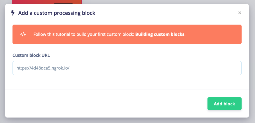

Adding a custom processing block from an ngrok URL

After you click Add block the block will show like any other processing block.

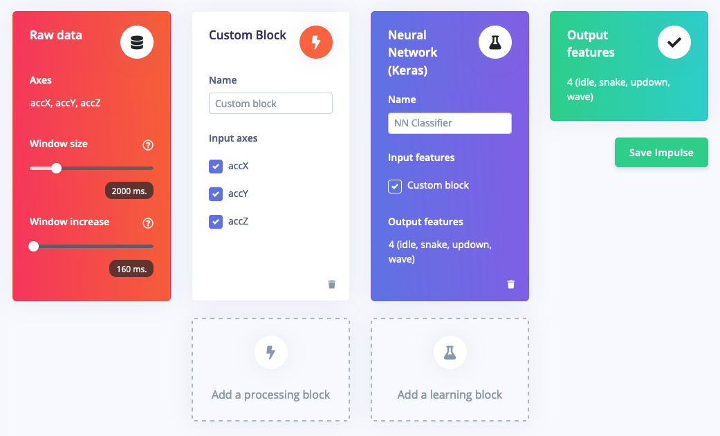
An impulse with a custom processing block and a neural network.

Add a learning bloc, then click Save impulse to store the impulse.

2. Adding configuration options

Processing blocks have configuration options which are rendered on the block parameter page. These could be filter configurations, scaling options, or control which visualizations are loaded. These options are defined in the parameters.json file. Let's add an option to smooth raw data. Open example-custom-processing-block-python/parameters.json and add a new section under parameters:

        {
            "group": "Filter",
            "items": [
                {
                    "name": "Smooth",
                    "value": false,
                    "type": "boolean",
                    "help": "Whether to smooth the data",
                    "param": "smooth"
                }
            ]
        }

Then, open example-custom-processing-block-python/dsp.py and replace its contents with:

import numpy as np

def generate_features(implementation_version, draw_graphs, raw_data, axes, sampling_freq, scale_axes, smooth):
    return { 'features': raw_data * scale_axes, 'graphs': [] }

Restart the Python script, and then click Custom block in the studio (in the navigation bar). You now have a new option 'Smooth'. Every time an option changes we'll re-run the block, but as we have not written any code to respond to these changes nothing will happen.

2.1 Customizing parameters

For the full documentation on customizing parameters, and a list of all configuration options; see Adding parameters to custom blocks.

3. Implementing smoothing and drawing graphs

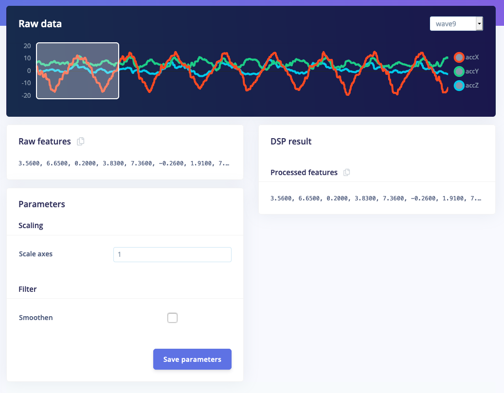
To show the user what is happening we can also draw visuals in the processing block. Right now we support graphs (linear and logarithmic) and arbitrary images. By showing a graph of the smoothed sample we can quickly identify what effect the smooth option has on the raw signal. Open dsp.py and replace the content with the following script. It contains a very basic smoothing algorithm and draws a graph:

import numpy as np

def smoothing(y, box_pts):
    box = np.ones(box_pts) / box_pts
    y_smooth = np.convolve(y, box, mode='same')
    return y_smooth

def generate_features(implementation_version, draw_graphs, raw_data, axes, sampling_freq, scale_axes, smooth):
    # features is a 1D array, reshape so we have a matrix with one raw per axis
    raw_data = raw_data.reshape(int(len(raw_data) / len(axes)), len(axes))

    features = []
    smoothed_graph = {}

    # split out the data from all axes
    for ax in range(0, len(axes)):
        X = []
        for ix in range(0, raw_data.shape[0]):
            X.append(raw_data[ix][ax])

        # X now contains only the current axis
        fx = np.array(X)

        # first scale the values
        fx = fx * scale_axes

        # if smoothing is enabled, do that
        if (smooth):
            fx = smoothing(fx, 5)

        # we save bandwidth by only drawing graphs when needed
        if (draw_graphs):
            smoothed_graph[axes[ax]] = list(fx)

        # we need to return a 1D array again, so flatten here again
        for f in fx:
            features.append(f)

    # draw the graph with time in the window on the Y axis, and the values on the X axes
    # note that the 'suggestedYMin/suggestedYMax' names are incorrect, they describe
    # the min/max of the X axis
    graphs = []
    if (draw_graphs):
        graphs.append({
            'name': 'Smoothed',
            'X': smoothed_graph,
            'y': np.linspace(0.0, raw_data.shape[0] * (1 / sampling_freq) * 1000, raw_data.shape[0] + 1).tolist(),
            'suggestedYMin': -20,
            'suggestedYMax': 20
        })

    return {
            'features': features,
            'graphs': graphs,
            'output_config': {
                # type can be 'flat', 'image' or 'spectrogram'
                'type': 'flat',
                'shape': {
                    # shape should be { width, height, channels } for image, { width, height } for spectrogram
                    'width': len(features)
                }
            }
        }

Restart the script, and click the Smooth toggle to observe the difference. Congratulations! You have just created your first custom processing block.

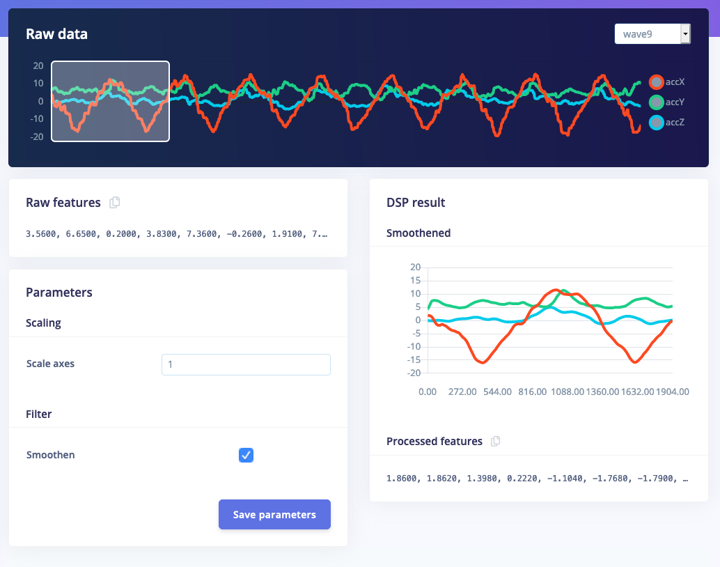
Custom processing block with a "smooth" option that shows a graph of the processed features.

3.1 Adding features to labels

If you extract set features from the signal, like the mean, that you that return, you can also label these features. These labels will be used in the feature explorer. To do so, add a labels array that contains strings that map back to the features you return (labels and features should have the same length).

4. Other type of graphs

In the previous step we drew a linear graph, but you can also draw logarithmic graphs or even full images. This is done through the type parameter:

4.1 Logarithmic graphs

This draws a graph with a logarithmic scale: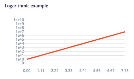

    graphs.append({
        'name': 'Logarithmic example',
        'X': {
            'Axis title': [ pow(10, i) for i in range(10) ]
        },
        'y': np.linspace(0, 10, 10).tolist(),
        'suggestedXMin': 0,
        'suggestedXMax': 10,
        'suggestedYMin': 0,
        'suggestedYMax': 1e+10,
        'type': 'logarithmic'
    })

4.2 Images

To show an image you should return the base64 encoded image and its MIME type. Here's how you draw a small PNG image: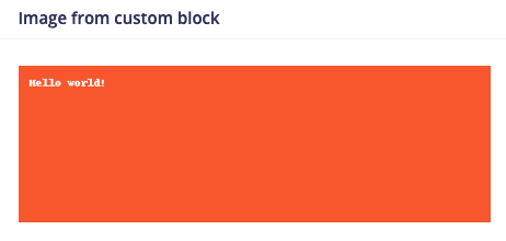

    from PIL import Image, ImageDraw, ImageFont, ImageFilter

    # create a new image, and draw some text on it
    im = Image.new ('RGB', (438, 146), (248, 86, 44))
    draw = ImageDraw.Draw(im)
    draw.text((10, 10), 'Hello world!', fill=(255, 255, 255))

    # save the image to a buffer, and base64 encode the buffer
    with io.BytesIO() as buf:
        im.save(buf, format='png', bbox_inches='tight', pad_inches=0)
        buf.seek(0)
        image = (base64.b64encode(buf.getvalue()).decode('ascii'))

        # append as a new graph
        graphs.append({
            'name': 'Image from custom block',
            'image': image,
            'imageMimeType': 'image/png',
            'type': 'image'
        })

4.3 Dimensionality reduction

If you output high-dimensional data (like a spectrogram or an image) you can enable dimensionality reduction for the feature explorer. This will run UMAP over the data to compress the features into three dimensions. To do so, set:

"visualization": "dimensionalityReduction"

On the info object in parameters.json.

4.4 Full documentation

For all options that you can return in a graph, see the Run DSP return types in the API documentation.

5. Running on device

Your custom block behaves exactly the same as any of the built-in blocks. You can process all your data, train neural networks or anomaly blocks, and validate that your model works.

However, we cannot automatically generate optimized native code for the block, like we do for built-in processing blocks, but we try to help you write this code as much as possible.

Export as a C++ Library:

• In the Edge Impulse platform, export your project as a C++ library.

• Choose the model type that suits your target device (quantized vs. float32).

Forward Declaration:

You don't need to add this part, it is automatically generated!

In the model-parameters/model_variables.h file of the exported C++ library, you can see a forward declaration for the custom DSP block you created.

For example:

int extract_my_preprocessing_features(signal_t *signal, matrix_t *output_matrix, void *config_ptr, const float frequency);

The name of that function comes from the cppType field in your custom DSP parameter.json. It takes your {cppType} and generates the following extract_{cppType}_features function.

Implement the Custom DSP Block:

In the main.cpp file of the C++ library, implement the extract_my_preprocessing_features block. This block should:

1. Call into the Edge Impulse SDK to generate features.

2. Execute the rest of the DSP block, including neural network inference.

For examples, have a look at our official DSP blocks implementations in our Inferencing C++ SDK

Also, please have a look at the video on the top of this page (around minute 25) where Jan explains how to implement your custom DSP block with your C++ library.

Compile and Run the App

• Copy a test sample's raw features into the features[] array in source/main.cpp

• Enter make -j in this directory to compile the project. If you encounter any OOM memory error try make -j4 (replace 4 with the number of cores available)

• Enter ./build/app to run the application

• Compare the output predictions to the predictions of the test sample in the Edge Impulse Studio.

6. Other resources

Blog post: Utilize Custom Processing Blocks in Your Image ML Pipelines

7. Conclusion

With good feature extraction you can make your machine learning models smaller and more reliable, which are both very important when you want to deploy your model on embedded devices. With custom processing blocks you can now develop new feature extraction pipelines straight from Edge Impulse. Whether you're following the latest research, want to implement proprietary algorithms, or are just exploring data.

For inspiration we have published all our own blocks here: edgeimpulse/processing-blocks. If you've made an interesting block that you think is valuable for the community, please let us know on the forums or by opening a pull request. We'd be happy to help write efficient native code for the block, and then publish it as a standard block!

Parameters.json format

This is the format for the parameters.json file:

type DSPBlockParametersJson = {
    version: 1,
    type: 'dsp',
    info: {
        type: string;
        title: string;
        author: string;
        description: string;
        name: string;
        preferConvolution: boolean;
        convolutionColumns?: 'axes' | string;
        convolutionKernelSize?: number;
        cppType: string;
        visualization: 'dimensionalityReduction' | undefined;
        experimental: boolean;
        hasTfliteImplementation: boolean; // whether we can fetch TFLite file for this DSP block
        latestImplementationVersion: number;
        hasImplementationVersion: boolean; // whether implementation version should be passed in (for custom blocks)
        hasFeatureImportance: boolean;
        hasAutoTune?: boolean;
        minimumVersionForAutotune?: number;
        usesState?: boolean; // Does the DSP block use feedback, do you need to keep the state object and pass it back in
        // Optional: named axes
        axes: {
            name: string,
            description: string,
            optional?: boolean,
        }[] | undefined;
        port?: number;
    },
    // see spec in https://docs.edgeimpulse.com/docs/tips-and-tricks/adding-parameters-to-custom-blocks
    parameters: DSPParameterItem[];
};

\