Only available on the Enterprise planThis feature is only available on the Enterprise plan. Review our plans and pricing or sign up for our free expert-led trial today.
Available as a synthetic data blockThe time-series data augmentation block is also available as a synthetic data block. The parameters and usage are the same across both block types. For more information, see the synthetic data documentation.
Overview
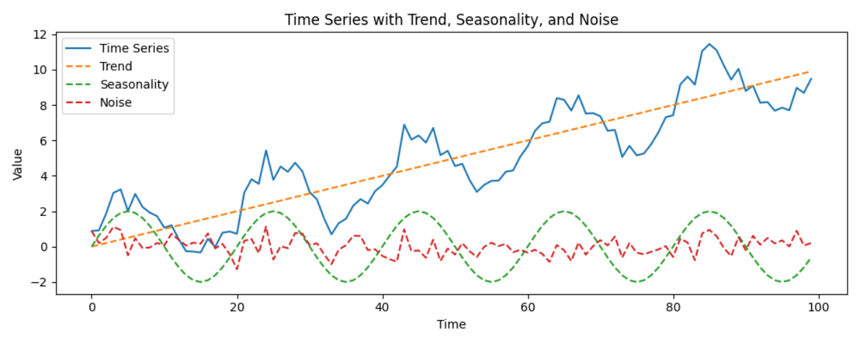
Time-series data is often composed of three main components:- Trend: Long-term progression (e.g., voltage drift in sensors)
- Seasonality: Repeating patterns (e.g., machine rotation cycles)
- Residual: Irregular short-term fluctuations (e.g., noise)
- Amplitude scaling (e.g., increase trend magnitude)
- Time scaling (e.g., compress or stretch the seasonal cycle)
- Synchronized slicing (reorder cycles of the seasonal component with smooth transitions)
- Use the trend from Series A
- Combine it with the seasonality from Series B
- Add the residual from Series C
Using the block in an organization
To use the time-series data augmentation block, navigate to your organization and go to the data transformation view, then select the Create job tab. From there, you can select the time-series data augmentation block from the transformation block dropdown menu.Block parameters
After selecting the time-series data augmentation block for a data transformation job, the block specific parameters will be shown. Each parameter is described below.Number of samples
The number of samples parameter specifies the number of additional data samples, per existing sample in your dataset, to generate from your original data. For example, if you have 100 samples in your dataset and you set this parameter to 4, 400 additional samples will be generated. The value must be a positive integer.Signal type
The signal type parameter allows you to specify whether the input time-series signal is periodic or not. If you are unsure, you can also select theunknown option. The option selected for this parameter aids the underlying algorithm in choosing the signal decomposition strategy.
Divergence
Instead of manually tuning multiple augmentation parameters, you can adjust a single divergence parameter. Behind the scenes, this parameter controls amplitude and time scaling, whether to apply slicing or remixing, and the degree of transformation per component. Higher divergence values lead to more pronounced changes, while lower values yield subtler variations. The divergence parameter accepts values between0.0 and 1.0.
Remix
The remix parameter is a boolean that allows you to specify whether to mix components across different series when generating augmented data. This is only applicable if your dataset contains multiple series from similar sources (e.g., different machines of the same origin). If set totrue, the augmentation process will randomly select components from different series to combine and create new samples, increasing the diversity of the generated data. If set to false, the augmentation will only transform components within the same series.
Signal column prefix
The signal column prefix parameter allows you to specify a prefix for the time-series signals that you wish to augment. This is useful when your dataset samples contain multiple different types of time-series data. For example, if your dataset samples contain both accelerometer and gyroscope data in the formataccel_x, accel_y, accel_z, gyro_x, gyro_y, gyro_z, you can specify accel as the signal column prefix to augment the accelerometer data. Only a single prefix can be specified.
Upsample factor
Parameter is conditionally shownThe upsample factor parameter is conditionally shown based on the selection for the signal type parameter. It will be shown if the signal type is set to
periodic.2, which will make the period contain 5 data points. An upsample factor of 1 means no upsampling is applied.
If your signal contains multiple periods, apply an upsample factor for the dominant period. You may need to experiment with different upsample factors to find the best setting for your specific use case.
Period range
Parameter is conditionally shownThe period range parameter is conditionally shown based on the selection for the signal type parameter. It will be shown if the signal type is set to
periodic.Best practices
Use high-quality input data
Use clean, representative examples; poor data leads to poor results. “Garbage in, garbage out” still applies.
Use consistent, single-label samples
This decomposition approach performs optimally when samples have uniform characteristics, with each labeled with a single class.
Start small and iterate
Begin with a small number of outputs and low divergence setting, and gradually explore the impact of tuning parameters.
Troubleshooting
No common issues have been identified thus far. If you encounter an issue, please reach out on the forum or, if you are on the Enterprise plan, through your support channels.