> ## Documentation Index
> Fetch the complete documentation index at: https://docs.edgeimpulse.com/llms.txt
> Use this file to discover all available pages before exploring further.
# Magnetic Vision - Seeed Wio Terminal
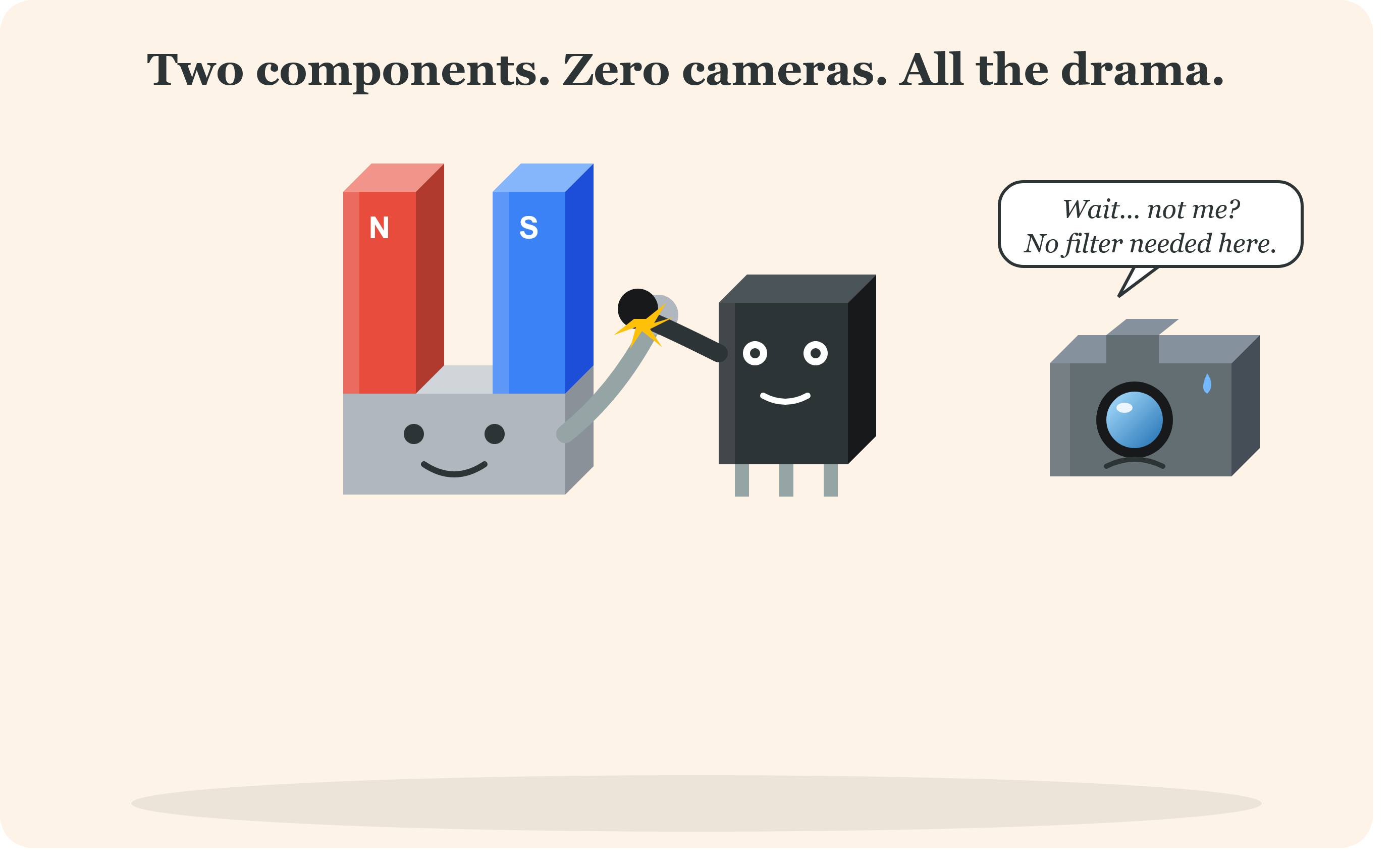
> Classify motion speed and patterns using a Hall-effect sensor and Edge Impulse. No camera required!
 Created By: Aula Jazmati
Public Project Links:
* [Experiment 1](https://studio.edgeimpulse.com/public/1112065/live)
* [Experiment 2](https://studio.edgeimpulse.com/public/1092905/live)
Demo Video links:
* [Experiment 1 - Live demo — take 1](https://www.youtube.com/shorts/AFlcssnsRv8?feature=share)
* [Experiment 1 - Live demo — take 2](https://www.youtube.com/shorts/ThNNQYDxOLE?feature=share)
* [Experiment 1 - FAST detection](https://www.youtube.com/shorts/ysYRykSbt78?feature=share)
* [Experiment 1 - SLOW / NO\_CAR detection](https://www.youtube.com/shorts/SpL6P7tqWLs?feature=share)
* [Experiment 2 - Live demo](https://www.youtube.com/shorts/MMltPG_8UW0?feature=share)
GitHub Repo:
[https://github.com/aula9/Magnetic-Vision-Teaching-AI-to-See-Motion-Without-a-Camera](https://github.com/aula9/Magnetic-Vision-Teaching-AI-to-See-Motion-Without-a-Camera)
## Introduction
What if a machine could understand motion without seeing it? This project explores whether a simple Hall-effect sensor can capture enough information about a moving object for a machine-learning model to recognize its motion — without any camera or computer vision.
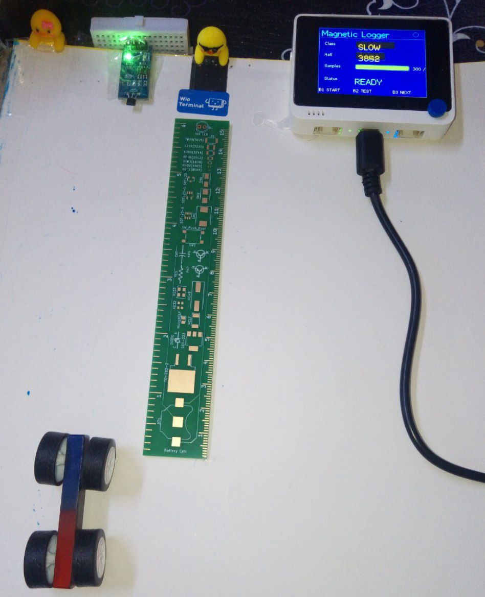
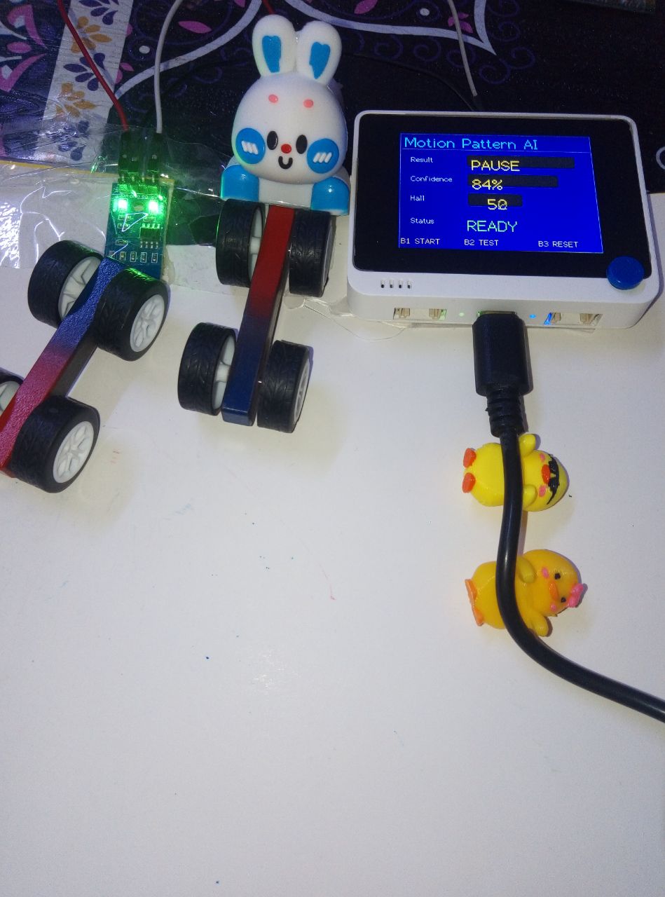
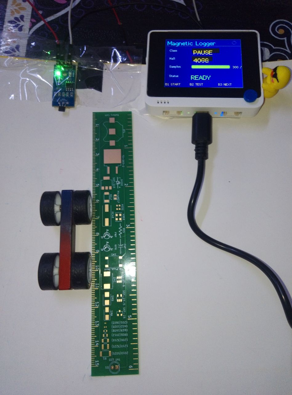
Using a Seeed Studio Wio Terminal, an A1302 linear Hall-effect sensor, and a small magnetic toy car, I recorded the magnetic field changes caused by the moving car.
Created By: Aula Jazmati
Public Project Links:
* [Experiment 1](https://studio.edgeimpulse.com/public/1112065/live)
* [Experiment 2](https://studio.edgeimpulse.com/public/1092905/live)
Demo Video links:
* [Experiment 1 - Live demo — take 1](https://www.youtube.com/shorts/AFlcssnsRv8?feature=share)
* [Experiment 1 - Live demo — take 2](https://www.youtube.com/shorts/ThNNQYDxOLE?feature=share)
* [Experiment 1 - FAST detection](https://www.youtube.com/shorts/ysYRykSbt78?feature=share)
* [Experiment 1 - SLOW / NO\_CAR detection](https://www.youtube.com/shorts/SpL6P7tqWLs?feature=share)
* [Experiment 2 - Live demo](https://www.youtube.com/shorts/MMltPG_8UW0?feature=share)
GitHub Repo:
[https://github.com/aula9/Magnetic-Vision-Teaching-AI-to-See-Motion-Without-a-Camera](https://github.com/aula9/Magnetic-Vision-Teaching-AI-to-See-Motion-Without-a-Camera)
## Introduction
What if a machine could understand motion without seeing it? This project explores whether a simple Hall-effect sensor can capture enough information about a moving object for a machine-learning model to recognize its motion — without any camera or computer vision.
Using a Seeed Studio Wio Terminal, an A1302 linear Hall-effect sensor, and a small magnetic toy car, I recorded the magnetic field changes caused by the moving car.
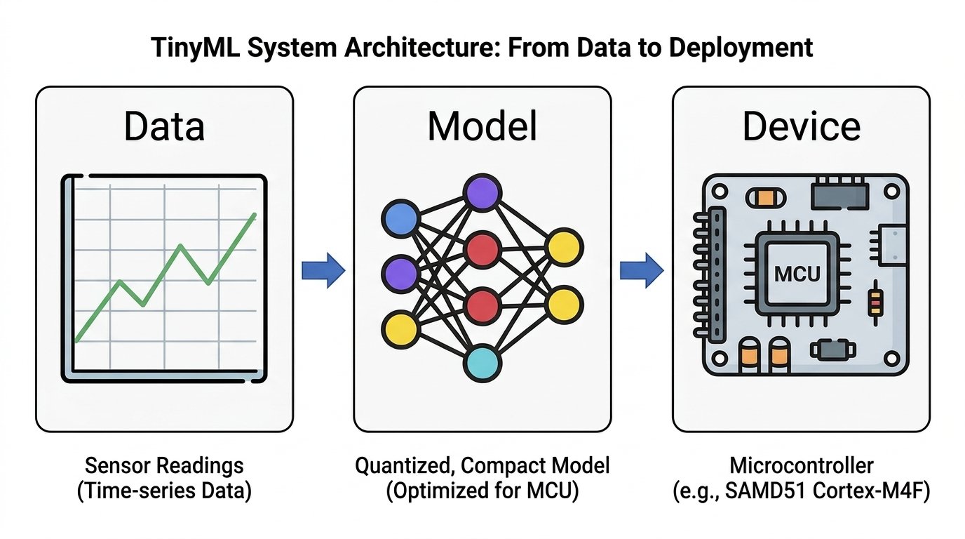 These changes were treated as a time-series signal, uploaded to Edge Impulse, and used to train two different machine-learning models that run entirely on-device.
The project contains two experiments:
* **Experiment 1**: Classify motion speed (FAST / SLOW / NO\_CAR) using statistical features.
* **Experiment 2**: Classify motion patterns (STRAIGHT / OSCILLATE / PAUSE) using a 1D CNN on raw signals.
The key finding: simple statistical features are sufficient for amplitude-based problems, but temporal patterns require more sophisticated, temporally-aware modeling.
## Requirements
### Hardware
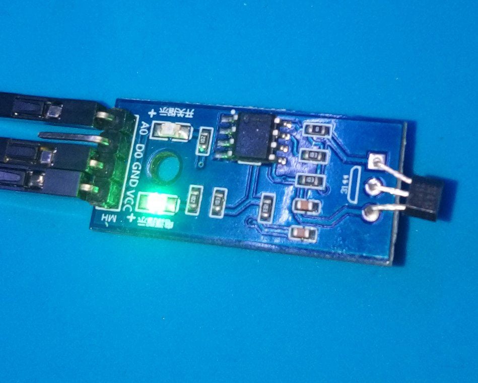
* 1 x Seeed Studio Wio Terminal (ARM Cortex-M4F, built-in LCD)
These changes were treated as a time-series signal, uploaded to Edge Impulse, and used to train two different machine-learning models that run entirely on-device.
The project contains two experiments:
* **Experiment 1**: Classify motion speed (FAST / SLOW / NO\_CAR) using statistical features.
* **Experiment 2**: Classify motion patterns (STRAIGHT / OSCILLATE / PAUSE) using a 1D CNN on raw signals.
The key finding: simple statistical features are sufficient for amplitude-based problems, but temporal patterns require more sophisticated, temporally-aware modeling.
## Requirements
### Hardware
* 1 x Seeed Studio Wio Terminal (ARM Cortex-M4F, built-in LCD)
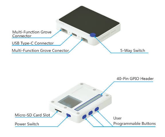 * 1 x A1302 Linear Hall-Effect Sensor
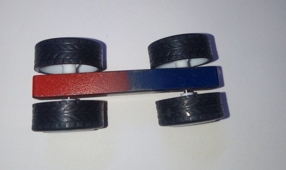
 * 1 x Magnetic toy car (from a magnetic science kit)
 * 3 x Jumper wires
* 1 x USB-C cable
### Software
* [Edge Impulse Studio](https://edgeimp.com/community26)
* [Arduino IDE](https://www.arduino.cc/en/software/) (v1.8.19 recommended)
* Python 3 (for the data logger)
* TFT\_eSPI library
### How It Works
The A1302 Hall-effect sensor is connected to the Wio Terminal's analog pin A0 (physical pin 13), powered at 3.3V for a wider ADC dynamic range. As the magnetic car moves near the sensor, the magnetic field changes, producing a time-varying analog signal.
* 3 x Jumper wires
* 1 x USB-C cable
### Software
* [Edge Impulse Studio](https://edgeimp.com/community26)
* [Arduino IDE](https://www.arduino.cc/en/software/) (v1.8.19 recommended)
* Python 3 (for the data logger)
* TFT\_eSPI library
### How It Works
The A1302 Hall-effect sensor is connected to the Wio Terminal's analog pin A0 (physical pin 13), powered at 3.3V for a wider ADC dynamic range. As the magnetic car moves near the sensor, the magnetic field changes, producing a time-varying analog signal.
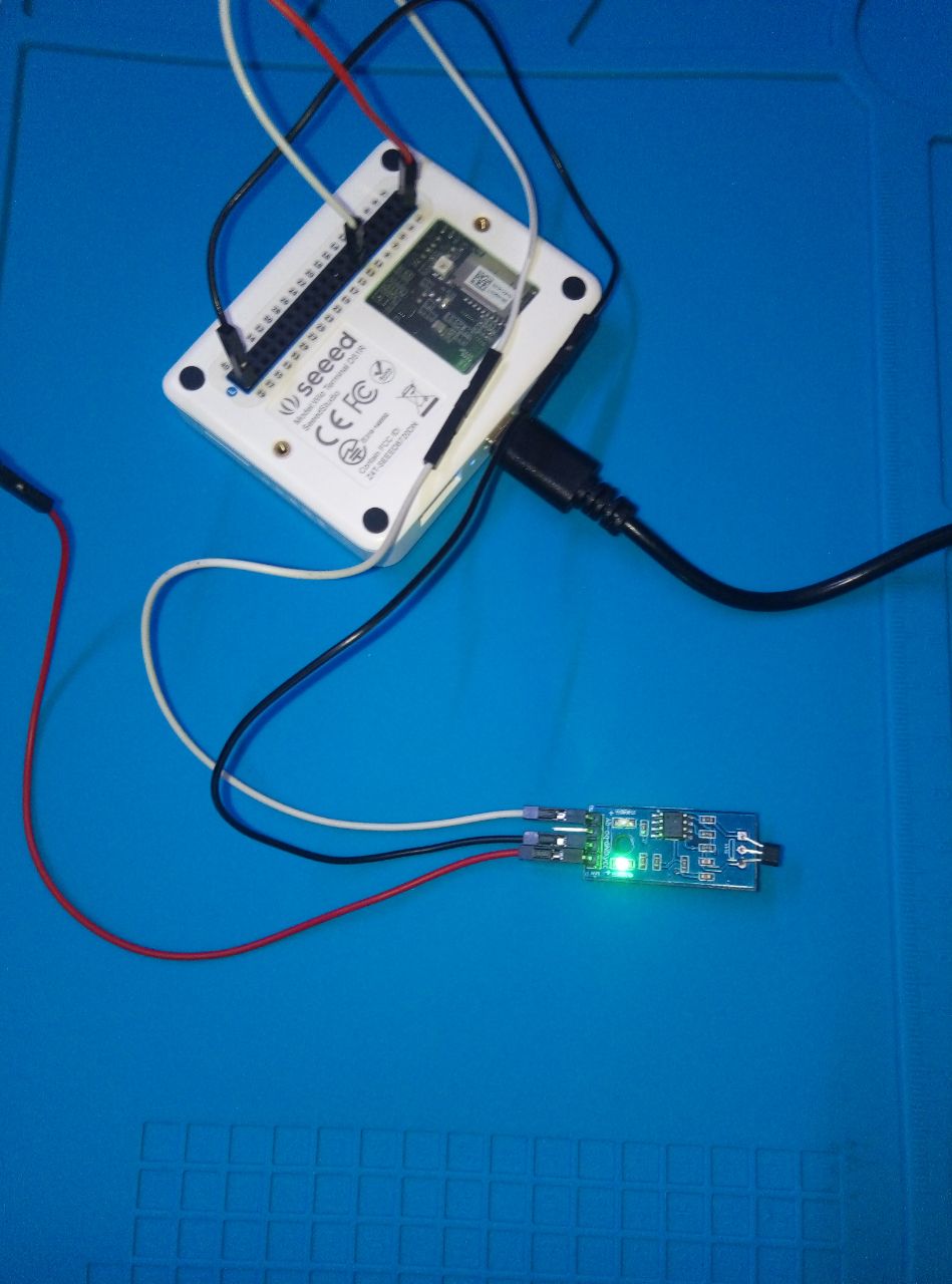 The Wio Terminal samples this signal at 100 Hz and streams the readings over USB Serial to a Python logger on a PC. The logger automatically organizes the recordings into class-labeled folders (e.g., \`dataset/FAST/\`, \`dataset/SLOW/\`).

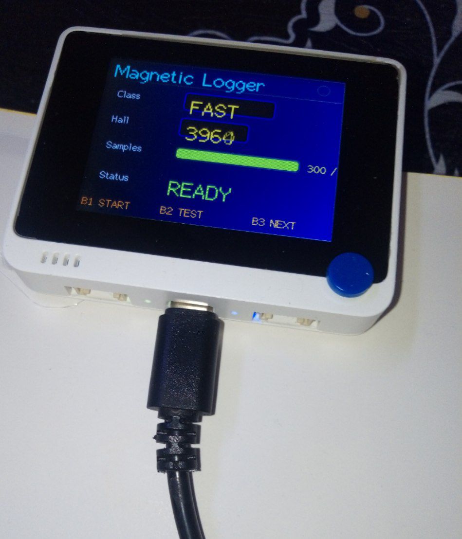
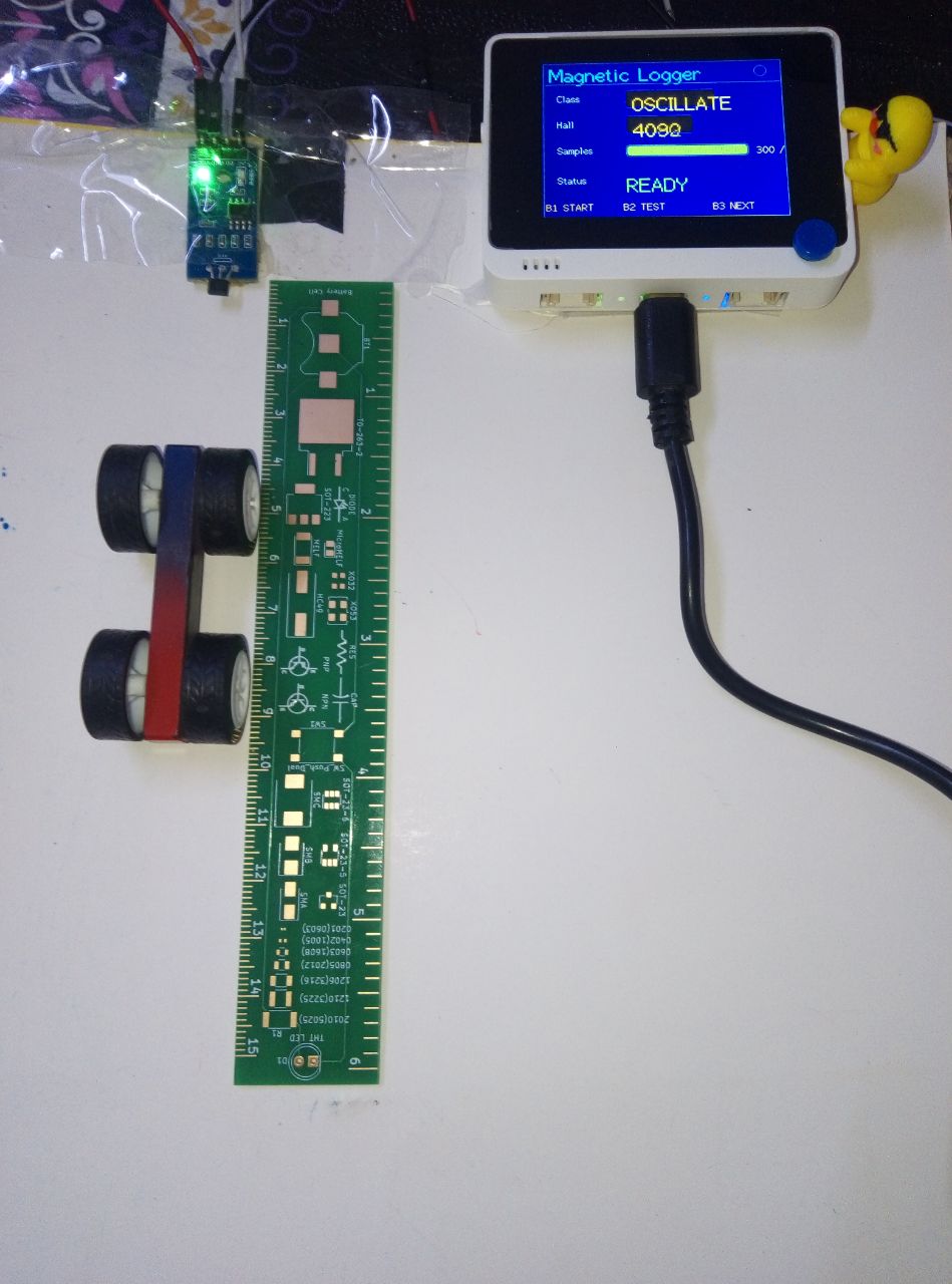
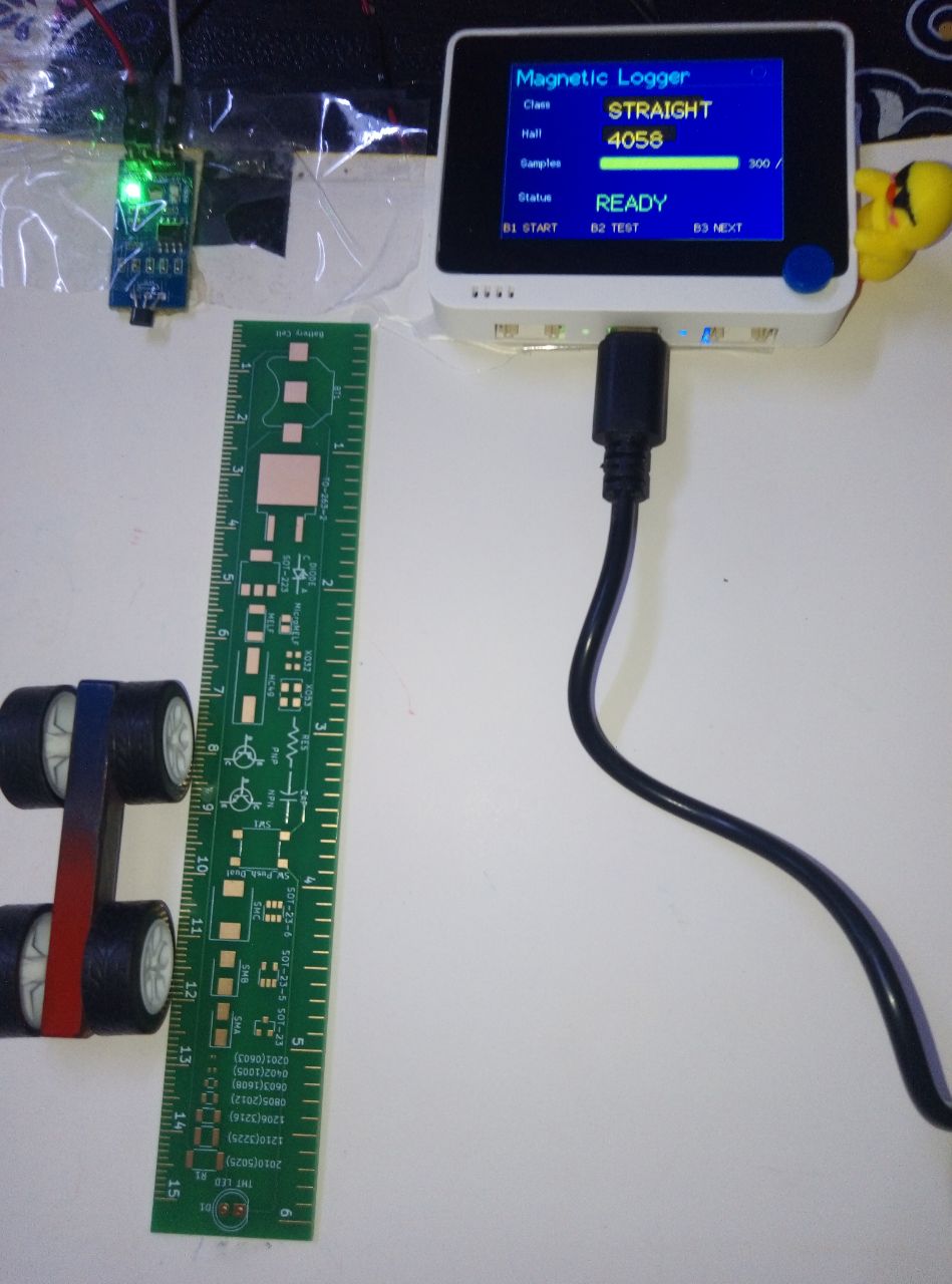
 For on-device inference, the trained model is deployed as an Arduino library. When the user presses button B1, the Wio Terminal records 3–6 seconds of sensor data, runs the impulse locally, and displays the predicted class and confidence on its built-in LCD — with no PC or cloud connection required.
## Data Preparation
A Python script (`logger.py`) listens to the serial port and automatically saves each recording as a CSV file with the format `timestamp, value`. The dataset is organized into class-labeled folders.
Two separate data collection firmwares were used:
### Experiment 1
Records 600 samples (6 seconds at 100 Hz) for three classes:
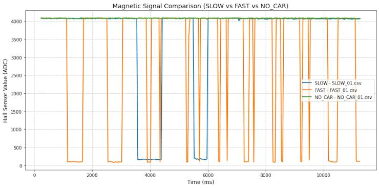
* `FAST`: car moves rapidly past the sensor
* `SLOW`: car moves slowly past the sensor
* `NO_CAR`: no car present near the sensor
For Experiment 1: 10 recordings per class (30 total).
For on-device inference, the trained model is deployed as an Arduino library. When the user presses button B1, the Wio Terminal records 3–6 seconds of sensor data, runs the impulse locally, and displays the predicted class and confidence on its built-in LCD — with no PC or cloud connection required.
## Data Preparation
A Python script (`logger.py`) listens to the serial port and automatically saves each recording as a CSV file with the format `timestamp, value`. The dataset is organized into class-labeled folders.
Two separate data collection firmwares were used:
### Experiment 1
Records 600 samples (6 seconds at 100 Hz) for three classes:
* `FAST`: car moves rapidly past the sensor
* `SLOW`: car moves slowly past the sensor
* `NO_CAR`: no car present near the sensor
For Experiment 1: 10 recordings per class (30 total).
 ### Experiment 2
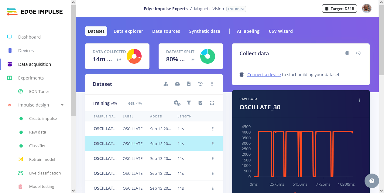
Records 300 samples (3 seconds at 100 Hz) for three classes:
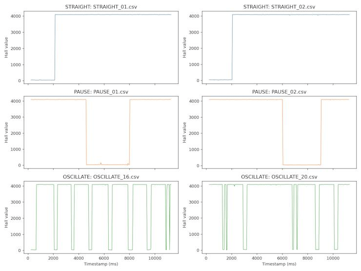
* `STRAIGHT`: steady movement in one direction
* `PAUSE`: movement, brief pause, then continuation
* `OSCILLATE`: back-and-forth movement within the recording window
For Experiment 2: 28–29 recordings per class (86 total).
### Experiment 2
Records 300 samples (3 seconds at 100 Hz) for three classes:
* `STRAIGHT`: steady movement in one direction
* `PAUSE`: movement, brief pause, then continuation
* `OSCILLATE`: back-and-forth movement within the recording window
For Experiment 2: 28–29 recordings per class (86 total).
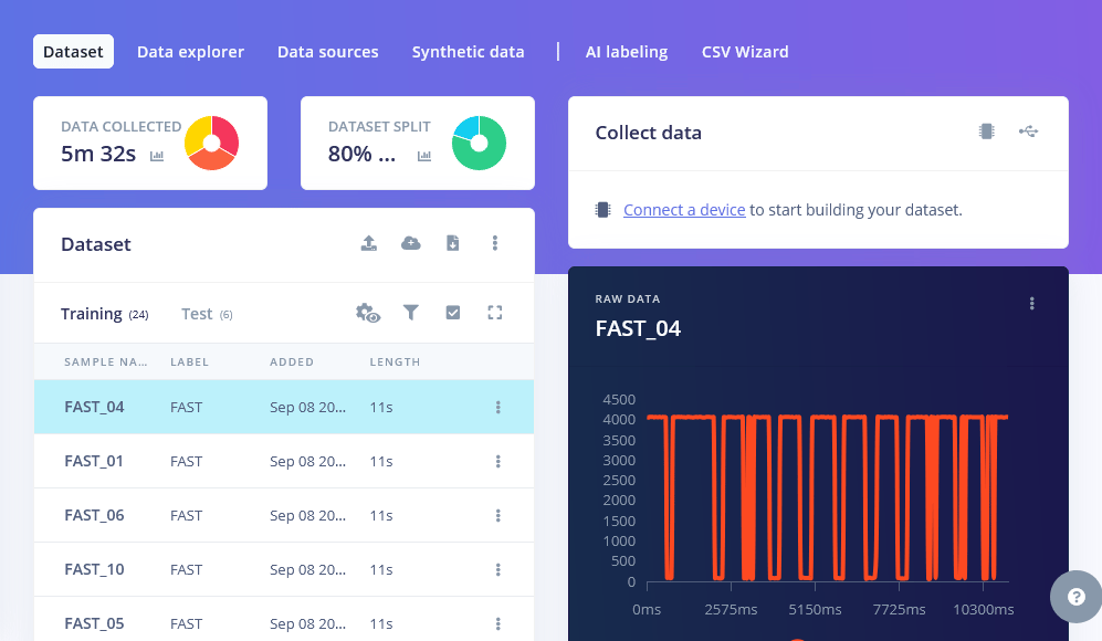
 All CSV files were uploaded to Edge Impulse using the Data Acquisition tool, with each file automatically labeled based on its folder name.
## Building the ML Model
### Experiment 1 — Speed Classification
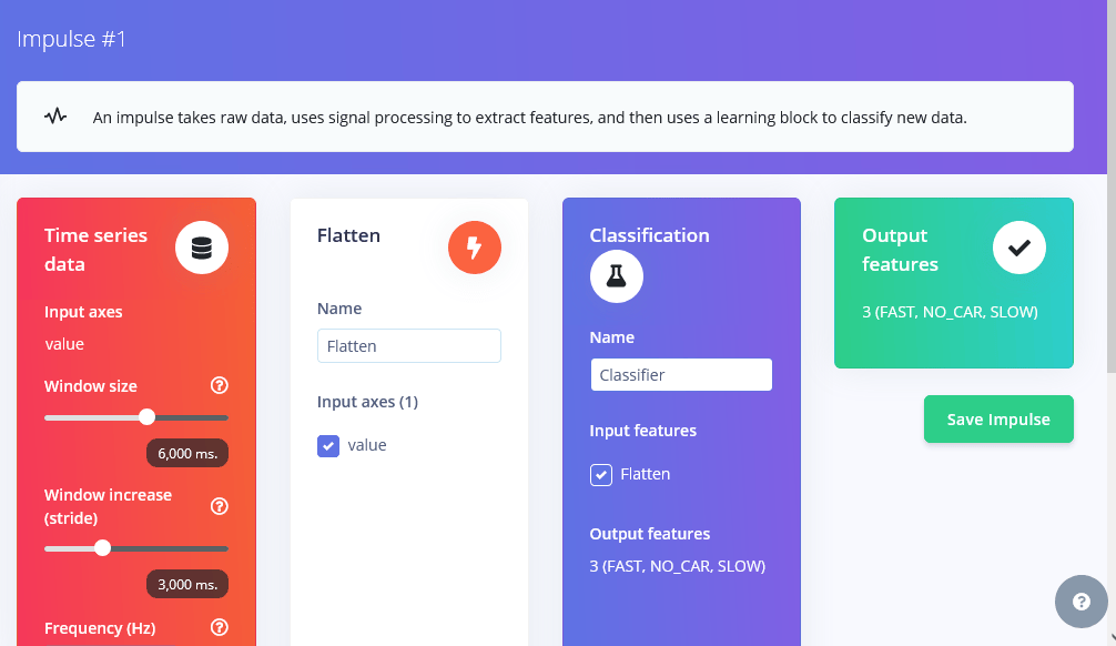
I designed an impulse with:
* Window size: 6000 ms (6 seconds at 100 Hz)
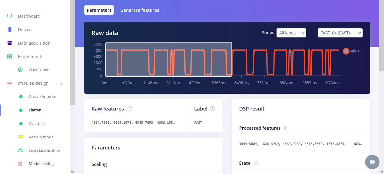
* Processing block: Flatten — extracts 7 statistical features per window:
Mean, Standard Deviation, Minimum, Maximum, RMS, Skewness, Kurtosis
* Learning block: Classification (Keras)
All CSV files were uploaded to Edge Impulse using the Data Acquisition tool, with each file automatically labeled based on its folder name.
## Building the ML Model
### Experiment 1 — Speed Classification
I designed an impulse with:
* Window size: 6000 ms (6 seconds at 100 Hz)
* Processing block: Flatten — extracts 7 statistical features per window:
Mean, Standard Deviation, Minimum, Maximum, RMS, Skewness, Kurtosis
* Learning block: Classification (Keras)
 #### Neural network architecture
* Input: 7 features
* Dense (20 neurons, ReLU) → Dense (10 neurons, ReLU) → Dropout (0.2)
* Output: 3 classes, Softmax
#### Neural network architecture
* Input: 7 features
* Dense (20 neurons, ReLU) → Dense (10 neurons, ReLU) → Dropout (0.2)
* Output: 3 classes, Softmax
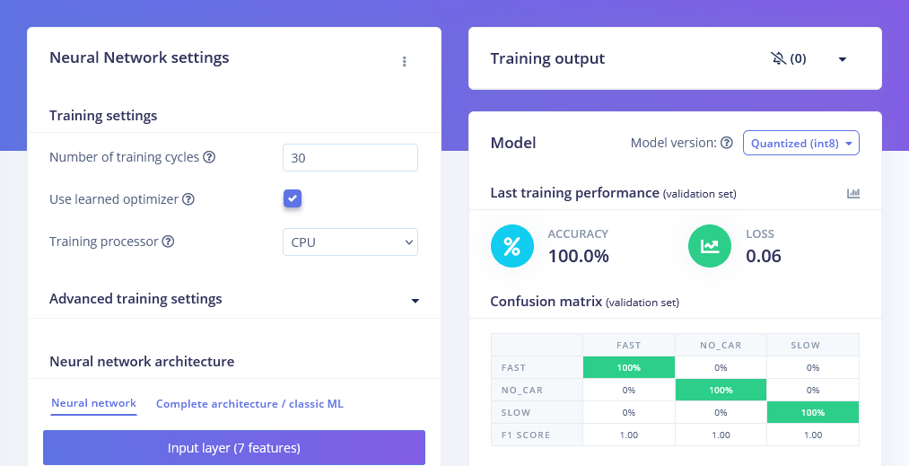 The model achieved 100% accuracy on both the validation and test sets.
Because the dataset is small and the setup is controlled, this result should be interpreted as a proof of concept rather than a general-purpose motion classifier.
The model achieved 100% accuracy on both the validation and test sets.
Because the dataset is small and the setup is controlled, this result should be interpreted as a proof of concept rather than a general-purpose motion classifier.
 ### Experiment 2 — Motion Pattern Classification
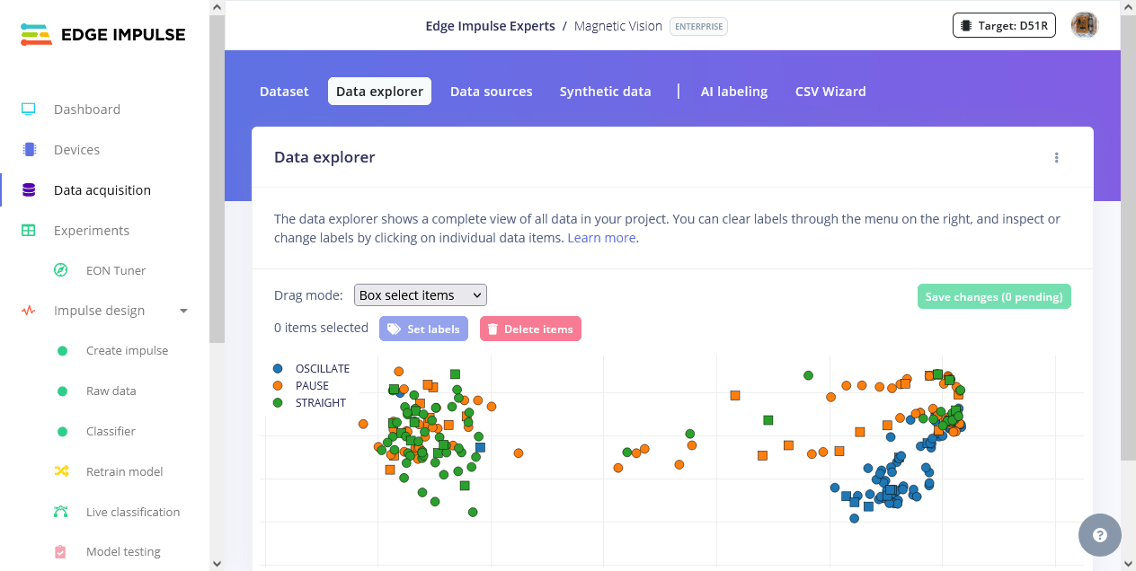
The same `Flatten` approach was tested first, but it only reached 61.5% accuracy confirming that statistical features alone cannot distinguish temporal patterns.
The approach was then changed to feed the raw 300-sample signal directly into a 1D Convolutional Neural Network.
### Experiment 2 — Motion Pattern Classification
The same `Flatten` approach was tested first, but it only reached 61.5% accuracy confirming that statistical features alone cannot distinguish temporal patterns.
The approach was then changed to feed the raw 300-sample signal directly into a 1D Convolutional Neural Network.
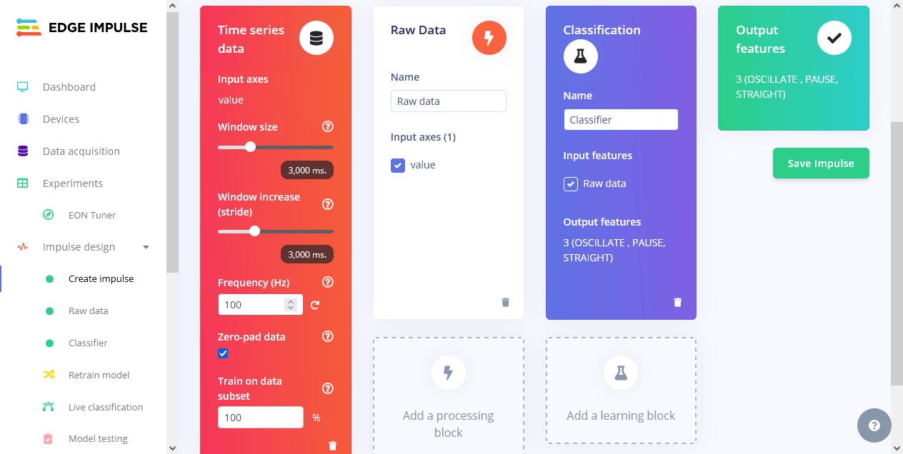
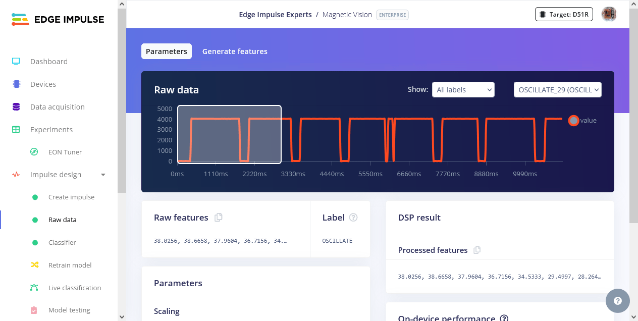
 * Window size: 3000 ms (3 seconds at 100 Hz)
* Processing block: Raw Data (300 samples)
* Learning block: Classification (Keras with 1D CNN)
* Window size: 3000 ms (3 seconds at 100 Hz)
* Processing block: Raw Data (300 samples)
* Learning block: Classification (Keras with 1D CNN)
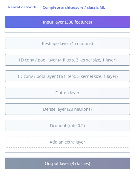
 #### Neural network architecture
* Input: 300 samples → Reshape (300 × 1)
* 1D Conv/Pool (4 filters, kernel 3) → 1D Conv/Pool (16 filters, kernel 3)
* Flatten → Dense (20, ReLU) → Dropout (0.2)
* Output: 3 classes, Softmax
#### Neural network architecture
* Input: 300 samples → Reshape (300 × 1)
* 1D Conv/Pool (4 filters, kernel 3) → 1D Conv/Pool (16 filters, kernel 3)
* Flatten → Dense (20, ReLU) → Dropout (0.2)
* Output: 3 classes, Softmax
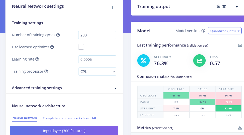
 The final results of the 2nd experiment is:
* Validation accuracy: 76.3%
* Test accuracy: 66.67%
The final results of the 2nd experiment is:
* Validation accuracy: 76.3%
* Test accuracy: 66.67%
 ### Deploying the Model
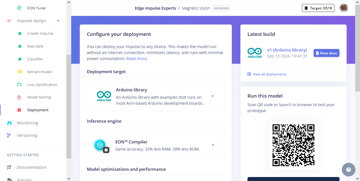
Both models were deployed as quantized (Int8) Arduino libraries from the Edge Impulse Deployment page. The Wio Terminal runs the impulse entirely on-device:
* Experiment 1 on-device performance: `< 1 ms` inference latency, `< 2 KB` RAM
* Experiment 2 on-device performance: `5 ms` inference latency, 13.8 KB RAM, 68.5 KB Flash
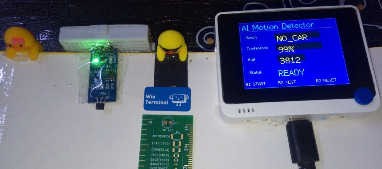
When the user presses B1, the Wio Terminal records the sensor data, runs the impulse locally, and displays the result instantly on its built-in screen. No PC, no cloud, and no Internet connection is required.
### Deploying the Model
Both models were deployed as quantized (Int8) Arduino libraries from the Edge Impulse Deployment page. The Wio Terminal runs the impulse entirely on-device:
* Experiment 1 on-device performance: `< 1 ms` inference latency, `< 2 KB` RAM
* Experiment 2 on-device performance: `5 ms` inference latency, 13.8 KB RAM, 68.5 KB Flash
When the user presses B1, the Wio Terminal records the sensor data, runs the impulse locally, and displays the result instantly on its built-in screen. No PC, no cloud, and no Internet connection is required.
 ## Conclusion
This project demonstrates that not all motion-recognition problems are equally suited to simple statistical feature extraction. While **Experiment 1** showed that speed classification can be solved almost perfectly with basic statistics (`Flatten`), **Experiment 2** proved that pattern classification requires more sophisticated, temporally-aware modeling (1D CNN on raw signals).
This is a meaningful finding in its own right: it shows precisely when simple embedded ML techniques are sufficient, and when a problem's underlying structure demands more advanced modeling. This is an important lesson for anyone building constrained, sensor-driven AI systems.
No camera. No images. Just a magnetic field, a sensor, and the right feature engineering.
## Conclusion
This project demonstrates that not all motion-recognition problems are equally suited to simple statistical feature extraction. While **Experiment 1** showed that speed classification can be solved almost perfectly with basic statistics (`Flatten`), **Experiment 2** proved that pattern classification requires more sophisticated, temporally-aware modeling (1D CNN on raw signals).
This is a meaningful finding in its own right: it shows precisely when simple embedded ML techniques are sufficient, and when a problem's underlying structure demands more advanced modeling. This is an important lesson for anyone building constrained, sensor-driven AI systems.
No camera. No images. Just a magnetic field, a sensor, and the right feature engineering.